This post covers Introduction to probability from Statistics for Engineers and Scientists by William Navidi.

Basic Ideas

• Random Variables

  • A random variable assigns a numerical value to each outcome in a sample space.

• Suppose that an electrical engineer has on hand six resistors. Three of them are labeled $10 \Omega$ and the other three are labeled $20\Omega$. The engineer wants to connect a $10 \Omega$ resistor and a $20 \Omega$resistor in series, to create a resistance of $30 \Omega$. Now suppose that in fact the three resistors labeled $10 \Omega$ have actual resistances of $9$, $10$, and $11 \Omega$, and that the three resistors labeled 20 Ω have actual resistances of $19$, $20$, and $21 \Omega$​​. The process of selecting one resistor of each type is an experiment whose sample space consists of nine equally likely outcomes. List the possible values of the random variable X, and find the probability of each of them.

• The function X, which assigns a numerical value to each outcome in the sample space, is a random variable.

• Random Variables and Populations

  • Discrete Random Variables

    • A random variable is discrete if its possible values form a discrete set. This means that if the possible values are arranged in order, there is a gap between each value and the next one. The set of possible values may be infinite; for example, the set of all integers and the set of all positive integers are both discrete sets.
    • Computer chips often contain surface imperfections. For a certain type of computer chip, $9\%$ contain no imperfections, $22\%$ contain $1$ imperfection, $26\%$ contain $2$ imperfections, $20\%$ contain $3$ imperfections, $12\%$ contain $4$​ imperfections, and the remaining $11\%$ contain $5$​ imperfections. Let Y represent the number of imperfections in a randomly chosen chip. What are the possible values for $Y$? Is $Y$ discrete or continuous? Find $P(Y = y)$ for each possible value $y$​​.

• The list of possible values of random variable X along with the probabilities for each, provide a complete description of the population from which $X$ is drawn. This description has a name—the probability mass function.

• The probability mass function of a discrete random variable X is the function $p(x) = P(X = x)$. The probability mass function is sometimes called the probability distribution.

• Note that if the values of the probability mass function are added over all the possible values of X, the sum is equal to 1

  

• The Cumulative Distribution Function of a Discrete Random Variable

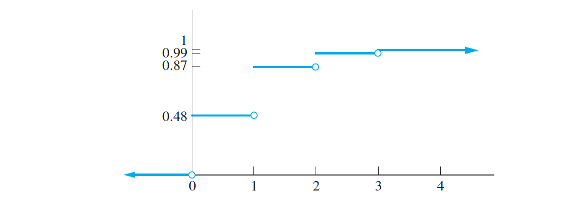
  • The probability mass function specifies the probability that a random variable is equal

    to a given value.

  • The cumulative distribution function of the random variable X is the function $F(x) = P(X ≤ x)$

  • Mean and Variance for Discrete Random Variables

    • The population mean of a discrete random variable can be thought of as the mean of

      a hypothetical sample that follows the probability distribution perfectly.

    • Let X be a discrete random variable with probability mass function $p(x) = P(X = x)$. The mean of X is given by $\mu_{X} =Σ_{x}xP(X = x)$ (where the sum is over all possible values of X).

  • The variance of $X$ is given by $\sigma_{X}^2 = \Sigma_{x} (x − \mu_{X})P(X = x)$​​​

  • A resistor in a certain circuit is specified to have a resistance in the range $99 \Omega–101 \Omega$. An engineer obtains two resistors. The probability that both of them meet the specificationis $0.36$, the probability that exactly one of them meets the specification is $0.48$, and the probability that neither of them meets the specification is $0.16$. Let $X$ represent the number of resistors that meet the specification. Find the probability mass function, and the mean, variance, and standard deviation of $X$.

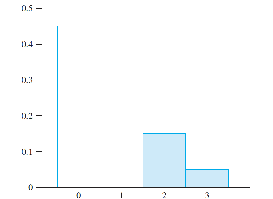
• • The Probability Histogram- When the possible values of a discrete random variable are evenly spaced, the probability mass function can be represented by a histogram,

• 

• Continuous Random Variables

  • A continuous random variable is defined to be a random variable whose probabilities are represented by areas under a curve. This curve is called the probability density function.

  • Let X be a continuous random variable with probability density function f (x). Let a and b be any two numbers, with a < b. Then the proportion of the population whose values of X lie between a and b is given by $\int_{a}^{b} f(x) \,dx$ , the area under the probability density function between a and b. This is the probability that the random variable X takes on a value between a and b.

  • Let X be a continuous random variable with probability density function f (x).

    Then $\int_{-\infty}^{\infty} f(x) \,dx$ = 1

  • The Cumulative Distribution Function of a Continuous Random Variable

    • F(x) = P(X ≤ x) = $\int_{-\infty}^{x} f(t) \,dt$

  • A hole is drilled in a sheet-metal component, and then a shaft is inserted through the hole. The shaft clearance is equal to the difference between the radius of the hole and the radius of the shaft. Let the random variable X denote the clearance, in millimeters.

​ The probability density function of X is \(p(x) = P(X = x) = \left\{\begin{array}{ll} {1.25(1-x^{4})} & 0 < x < 1, \\ 0 & otherwise \end{array}\right.\) ​

​ Components with clearances larger than 0.8 mm must be scrapped. What proportion of components are scrapped?

• Mean and Variance for Continuous Random Variables

  • Let X be a continuous random variable with probability density function f (x).

    Then the mean of X is given by

    $ \mu_{X} = = \int_{-\infty}^{\infty} xf(x) \,dx$

  • The mean of X is sometimes called the expectation, or expected value, of X and

    may also be denoted by E(X) or by 𝜇.

  • The variance of X is given by $ \sigma_{X} = \int_{-\infty}^{\infty} (x-\mu_{X})^2 f(x) \,dx$

  • The Population Median and Percentiles

    • Let X be a continuous random variable with probability mass function f (x) and

      cumulative distribution function F(x). The median of X is the point $x_{m}$ that solves the equation

      $F(x_{m}) = P(X ≤ x_{m}) = \int_{-\infty}^{ x_{p}} f (x) dx = .50$

  • If p is any number between 0 and 100, the pth percentile is the point $x_{p}$ that solves the equation $F(x_{p}) = P(X ≤ x_{p}) = \int_{-\infty}^{ x_{p}} f (x) dx = p∕100$.

    • The median is the 50th percentile.

• Chebyshev’s Inequality

  • Let X be a random variable with mean $𝜇_{X}$ and standard deviation $𝜎_{X}$. Then

    $P(\mid X − 𝜇_{X} \mid ≥ k𝜎_{X}) ≤ 1/k^2$

  • The mean of a random variable is a measure of the center of its distribution. and the

    standard deviation is a measure of the spread.

  • Chebyshev’s inequality relates the mean and the standard deviation by providing a bound on the probability that a random variable takes on a value that differs from its mean by more than a given multiple of its standard deviation

  • The length of a rivet manufactured by a certain process has mean $\mu_{X} = 50 ~ mm$ and standard deviation $\sigma_{X} = 0.45 ~ mm$. What is the largest possible value for the probability that the length of the rivet is outside the interval $49.1–50.9 ~ mm$?

Derivation of the Alternate Formula for the Variance

$ \sigma_X^2 = \sum_\limits{x}{} (x-\mu_X)^2 P(X=x) $

Multiplying out $(x − 𝜇_{X})^{2}$, we obtain

$ \sigma_X^2 = \sum_\limits{x}{} (x^2- 2x \mu_{X} + \mu_X^2) P(X=x) $

Distributing the term $P(X = x)$ over the terms in the parentheses yields

$ \sigma_X^2 = \sum_\limits{x}{} x^2P(X=x) - 2\mu_{X} \sum_\limits{x}{} x P(X=x)+ \mu_X^2 \sum_\limits{x}{} P(X=x) $

Summing the terms separately,

$ \sigma_X^2 = \sum_\limits{x}{} x^2P(X=x) - 2\mu_{X} \sum_\limits{x}{} x P(X=x)+ \mu_X^2 \sum_\limits{x}{} P(X=x) $

Now

$ 2\mu_{X} \sum_\limits{x}{} x P(X=x) = 2𝜇_{X}𝜇_{X} = 2𝜇^{2}_{X} $, and

$ \mu_X^2 \sum_\limits{x}{} P(X=x) = \mu_X^2 (1) = \mu_X^2 $

Substituting yields

$ \sigma_X^2 = \sum_\limits{x} x^2P(X=x) - 2\mu_X^2 + \mu_X^2 $

We conclude that

$ \sigma_X^2 = \sum_\limits{x}{} x^2P(X=x) - \mu_X^2 $

To derive the alternate formula for the variance of a continuous random variable, the same steps may be used; replacing

$Σ_{x}$ with $\int^{\infty}_{−\infty}$, and $P(X =x)$ with $f (x) dx$.