This post covers Introduction to probability from Statistics for Engineers and Scientists by William Navidi.

Basic Ideas

Statistical inference involves drawing a sample from a population and analyzing the sample data to learn about the population. Some of well known distributions are standard functions which are appropriate under particular conditions.

• The Binomial Distribution

• A trial that can result in one of two outcomes. One outcome is labeled “success,” and the other outcome is labeled “failure.” The probability of success is denoted by p. The probability of failure is therefore 1−p. Such a trial is called a Bernoulli trial with success probability p.

• If $ X \sim Bernoulli(p)$, then

  • $𝜇_{X} = p $
  • $𝜎 _{X}^2 = p(1 − p) $

Theoram: Prove that $𝜇_{X} = p $

Proof: Let X be a discrete random variable with probability mass function p(x) = P(X = x).

The mean of X is given by

​ $𝜇_{X} =ΣxP(X = x)$

where the sum is over all possible values of X.

If $X ∼ Bernoulli(p)$, then,

​ $𝜇_{X} = (0)(1 − p) + (1)(p) = p$

• If a total of n Bernoulli trials are conducted, and

  • The trials are independent
  • Each trial has the same success probability p
  • X is the number of successes in the n trials

  then X has the binomial distribution with parameters n and p, denoted$ X \sim Bin(n, p)$.

• Probability Mass Function of a Binomial Random Variable

  • the sample items may be treated as independent if the population is very large compared to the size of the sample

  • When the population of items is large compared to the number sampled, these Bernoulli trials are nearly independent, and the number of successes among them has, for all practical purposes, a binomial distribution

  • if the sample size is no more than $5\%$ of the population, the binomial distribution may

    be used to model the number of successes.

  • If $X \sim Bin(n, p)$, the probability mass function of X is \(p(x) = P(X = x) = \left\{ \begin{array}{ll} \frac{n!}{k!(n-k)!} p^x (1 − p)^{(n−x)} & x = 0, 1, \ldots , n \\ 0 & otherwise \end{array}\right.\)

• A lot contains several thousand components, $10\%$ of which are defective. Seven components are sampled from the lot. Let X represent the number of defective components in the sample. What is the distribution of X?

• A fair die is rolled eight times. Find the probability that no more than $2$ sixes come up.

• 

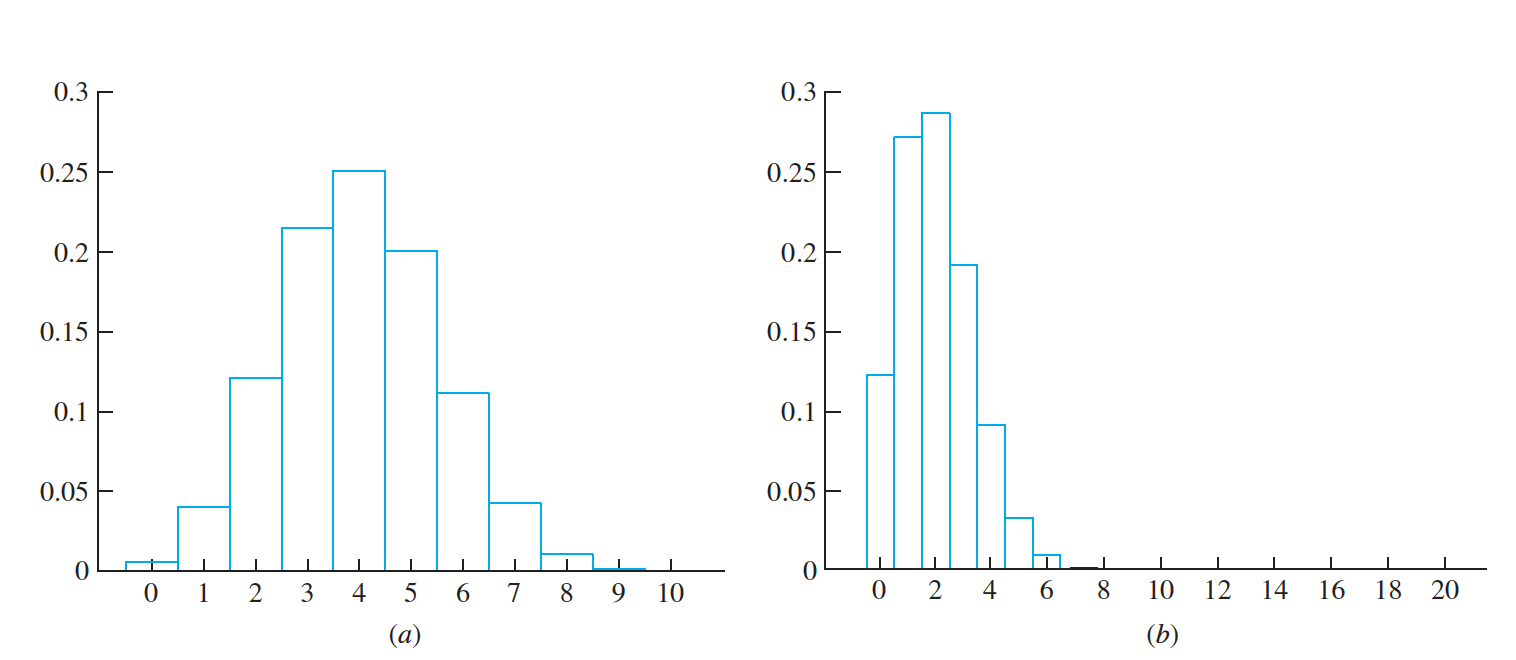
  ​ (a) The $ Bin(10, 0.4)$ probability histogram. (b) The $ Bin(20, 0.1)$ probability histogram.

  • A Binomial Random Variable Is a Sum of Bernoulli Random Variables

    • sampling a single value from a Bin(n, p) population is equivalent to drawing a sample of size n from a Bernoulli(p) population, and then summing the sample values

      • Assume n independent Bernoulli trials are conducted, each with success probability $p$. Let $Y_{1}, \ldots, Y_{n}$ be defined as follows: $Y_{i} = 1$ if the $i^{th}$ trial results in success, and $Y_{i} = 0$ otherwise.
      • Then each of the random variables $Y_i$ has the $Bernoulli(p)$ distribution. Now, let $X$ represent the number of successes among the $n$ trials. Then $X ∼ Bin(n, p)$. Since each $Y_i$ is either $0$ or $1$, the sum $Y_{1}+ \ldots + Y_{n}$ is equal to the number of the $Y_i$ that have the value 1, which is the number of successes among the n trials.
      • Therefore $X = Y_{1}+ \ldots + Y_{n}$. This shows that a binomial random variable can be expressed as a sum of Bernoulli random variables.
      • Put another way, sampling a single value from a $Bin(n, p)$ population is equivalent to drawing a sample of size n from a $Bernoulli(p)$ population, and then summing the sample values.

  • The Mean and Variance of a Binomial Random Variable

• If $X \sim Bin(n, p)$, then the mean and variance of X are given by $𝜇_X = np$ and $𝜎^2_{X}= np(1 − p)$

• Using a Sample Proportion to Estimate a Success Probability

  • $\hat{p} = \frac {number ~of ~successes}{ number~ of ~trials}= \frac{X}{n}$
    • conduct n independent trials and count the number X of successes

  • A quality engineer is testing the calibration of a machine that packs ice cream into containers. In a sample of $20$ containers, $3$ are underfilled. Estimate the probability $p$ that the machine underfills a container.

    • we must compute its bias and its uncertainty

    • If $X$ is a random variable and $a$ is a constant, then $\mu_{aX} = a\mu_{X}$

    • The bias is the difference $ \hat{\mu_p} − p $.

    • Since $ \hat{\mu_p}= \frac{X}{n} $, Since $\hat{\mu_p} = p $, $ \hat{\mu}_{p} $ is unbiased;

    • in other words, its bias is $0$.

    • Uncertainty in the Sample Proportion

      • If $X ∼ Bin(n, p)$, then the sample proportion $ \hat{p} = X∕n$ is used to estimate the

        success probability p.

        • $\hat{p}$ is unbiased.

      • The uncertainty in $\hat{p}$ is

      ​ $ \sigma_{\hat{p}} = \sigma_{\frac{X}{n}} = \frac{𝜎_{X}}{n} $

      ​ $= \frac{\sqrt{np(1 − p)}}{n}=\sqrt{\frac{p(1 − p)}{n}}$

      In practice, when computing $\hat{\sigma_{p}}$, we substitute $\hat{\sigma_{p}}$for $p$, since $p$ is unknown.

• In a sample of $100$ newly manufactured automobile tires, $7$ are found to have minor flaws in the tread. If four newlymanufactured tires are selected at random and installed on a car, estimate the probability that none of the four tires have a flaw, and find the uncertainty in this estimate.