Two independent samples
Published:
This post covers Introduction to probability from Statistics for Engineers and Scientists by William Navidi.
Basic Ideas
Confidence Intervals for the Difference Between Two Means
The data will consist of two samples, one from each population.
We will compute the difference of the sample means and the standard deviation of that difference.
Then a simple modification of expression will provide the confidence interval
Let X and Y be independent, with $ X \sim N (\mu_X, \sigma^2_X) $ and $ Y \sim N (\mu_Y, \sigma^2_Y) $
Then
$ X + Y \sim N (\mu_X + \mu_Y, \sigma^2_X + \sigma^2_Y) $
$ X - Y \sim N (\mu_X - \mu_Y, \sigma^2_X + \sigma^2_Y) $
How to construct a confidence interval for the difference between two population means.
- As an example, how to show that a new design developed is thought to last longer than an old design.
- We have a simple random sample $X_1,\ldots, X_{144}$ of lifetimes of new lightbulbs. The sample mean is $ \overline X = 578$ and the sample standard deviation is $s_X = 22$. We have another simple random sample $Y_1,…, Y_{64}$ of lifetimes of old lightbulbs. This sample has mean $ \overline Y = 551$ and standard deviation $s_Y = 33$. The population means and standard deviations are unknown.
Let $X_1,…, X_{n_X}$ be a large random sample of size $n_X$ from a population with mean $𝜇_X$ and standard deviation $\sigma_X$, and let $Y_1,…, Y_{n_Y}$ be a large random sample of size $n_Y$ from a population with mean $𝜇_Y$ and standard deviation $𝜎_Y$. If the two samples are independent, then a level $100(1 − 𝛼)\%$ confidence interval
for $𝜇_X − 𝜇_Y$ is $ \overline X − \overline Y \pm z_{ \alpha ∕2}\sqrt {\frac {𝜎^2_X}{n_X}+ \frac {𝜎^2_Y}{n_Y}}$
When the values of $𝜎_X$ and $𝜎_Y$ are unknown, they can be replaced with the sample standard deviations $s_X$ and $s_Y$.
Chemical analyses of soil taken from a farm in Western Australia. Fifty specimens were each taken at depths $50$ and $250$ cm. At a depth of $50$ cm, the average $NO_3$ concentration (in mg/L) was $88.5$ with a standard deviation of $49.4$. At a depth of $250$ cm, the average concentration was $110.6$ with a standard deviation of $51.5$. Find a $95\%$ confidence interval for the difference between the $NO_3$ concentrations at the two depths.
Confidence Intervals for the Difference Between Two Proportions
In a Bernoulli population, the mean is equal to the success probability $p$, which is the proportion of successes in the population. When independent trials are performed from each of two Bernoulli populations, we can use methods similar to those presented for confidence Intervals for the difference between two means
Eighteen of $60$ light trucks produced on assembly line $A$ had a defect in the steering
mechanism, which needed to be repaired before shipment. Only $16$ of $90$ trucks produced on assembly line $B$ had this defect. Assume that these trucks can be considered to be two independent simple random samples from the trucks manufactured on the twoassembly lines.
We wish to find a $95\%$ confidence interval for the difference between the. proportions of trucks with this defect on the two assembly lines.
- Let $X$ represent the number of trucks in the sample from line $A$ that had defects, and let $Y$ represent the corresponding number from line $B$. Then $X$ is a binomial random variable with $n_{X} = 60$ trials and success probability $p_X$, and $Y$ is a binomial random variable with $n_Y = 90$ trials and success probability $p_Y$ . The sample proportions are $ \hat p_X$ and ̂$ \hat p_Y$.
- In this example the observed values are $X = 18$, $Y = 16$, $ \hat p_X = \frac{18}{60}$, and $ \hat p_Y = \frac{16}{90}$
Let $p_X$ represent the proportion of trucks in the population from line $A$ that had the defect, and let $p_Y$ represent the corresponding proportion from line $B$. The values of $p_X$ and $p_Y$ are unknown. We wish to find a $95\%$ confidence interval for $p_X − p_Y$ .
Since the sample sizes are large, it follows from the Central Limit Theorem that $ \hat p_X$ and $ \hat p_Y$ are both approximately normally distributed with means $p_X$ and $p_Y$ and standard deviations $ \hat \sigma_X = \sqrt{ \frac {p_X( 1 − p_X)}{n_X}}$ and $ \hat \sigma_Y = \sqrt{ \frac {p_Y( 1 − p_Y)}{n_Y}}$.
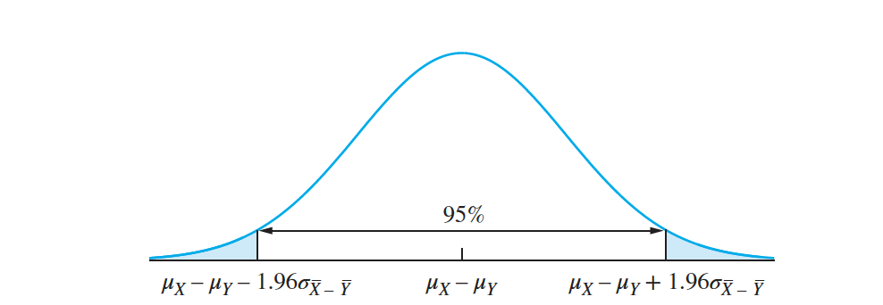
We conclude that for $95\%$ of all possible samples, the difference $p_X − p_Y$ satisfies the following inequality:
$ \hat p_X − \hat p_Y − 1.96 \sqrt{ \frac {p_X( 1 − p_X)}{n_X} + \frac {p_Y( 1 − p_Y)}{n_Y}}$ < $p_X − p_Y$ < $ \hat p_X − \hat p_Y + 1.96 \sqrt{ \frac {p_X( 1 − p_X)}{n_X} + \frac {p_Y( 1 − p_Y)}{n_Y}}$
The quantity $ \frac {p_X(1 − p_X)}{n_X} + \frac {p_Y (1 − p_Y )}{n_Y}$ depends on the unknown true values $p_X$ and $p_Y$.
It turns out that replacing the population proportions with the sample proportions tends to make the confidence interval too short in some cases, even for some fairly large sample sizes.
Recent research, involving simulation studies, has shown that this effect can be largely compensated for by slightly modifying $n_X$, $n_Y$, $p_X$, and $p_Y$.
Define $ \overline {n_X} = n_X + 2 $, $ \overline n_Y = n_Y + 2$, $ \overline p_X = \frac{ (X + 1)}{\overline n_X}$, and $ \overline p_Y = \frac {(Y + 1)}{\overline n_Y}$ .
$ \overline p_X − \overline p_Y − z_{\frac{\alpha}{2}} \sqrt{ \frac {\overline p_X( 1 − \overline p_X)}{\overline n_X} + \frac {\overline p_Y( 1 − \overline p_Y)}{\overline n_Y}} \overline p _X − \overline p_Y < \overline p_X − \overline p_Y $
$\overline p_X − \overline p_Y < \overline p_X − \overline p_Y + z_{\frac{\alpha}{2}} \sqrt{ \frac { \overline p_X( 1 − \overline p_X)}{\overline n_X} + \frac { \overline p_Y( 1 − \overline p_Y)}{\overline n_Y}}$
In this example $ \overline n_X = 62,\overline n_Y = 92,\overline p_X = 19∕62 = 0.3065$, and $ \overline p_Y = 17∕92 = 0.1848$. We thus obtain
$0.3065 − 0.1848 \pm 0.1395, or (−0.0178, 0.2612)$.
In a sample of $16,611$ men, $2350$ said they had used e-cigarettes, and in a sample of $17,745$ women, $1929$ said they had used them. Find a $95\%$ confidence interval for the difference between the proportions of men and women who have used e-cigarettes.
- Small-Sample Confidence Intervals for the Difference Between Two Means
The Student’s t distribution can be used in some cases where samples are small, and thus, where the Central Limit Theorem does not apply.
If $X_1,…, X_{n_X}$ is a sample of size $n_X$ from a normal population with mean $𝜇_X$ and $Y_1,…, Y_{n_Y}$ is a sample of size $n_Y$ from a normal population with mean $𝜇_Y$ , then the quantity
$(\overline X − \overline Y) − (\mu_X − \mu_Y ) \sqrt{ \frac{ s^2_X }{n_X} + \frac {s^2_Y}{n_Y}}$
has an approximate Student’s t distribution. The number of degrees of freedom to use for this distribution is given by
$𝜈 = \frac {(\frac {s^2_X}{ n_X} + \frac {s^2_Y} {n_Y })^2} {\frac {(\frac {s^2_X}{n_X})^2} {n_X − 1} + \frac {(\frac {s^2_Y}{n_Y} )^2} {n_Y − 1}}$
rounded down to the nearest integer.
We present an example.
A sample of $6$ welds of one type had an average ultimate testing strength (in ksi) of $83.2$ and a standard deviation of $5.2$, and a sample of $10$ welds of another type had an average strength of $71.3$ and a standard deviation of $3.1$. Assume that both sets of welds are random samples from normal populations. We wish to find a $95\%$ confidence interval for the difference between the mean strengths of the two types of welds.
Substituting $s_X = 5.2, s_Y = 3.1, n_X = 6, n_Y = 10$ into Equation for $\nu$ yields
$𝜈 =\frac{(\frac {5.2^2}{6}+ \frac {3.1^2}{10})^2}{ \frac {(\frac {5.2^2}{6})^2} 5+ \frac {(\frac {3.1^2}{10})^2}9}$
= 7.18 ≈ 7
It follows that for $95\%$ of all the samples that might have been chosen
$−2.365 < \frac {(\overline X − \overline Y) − (𝜇_X − 𝜇_Y )}{ \sqrt {s^2_X∕6 + s^2_Y∕10}} < 2.365$

Substituting $ \overline X = 83.2, \overline Y = 71.3, s_X = 5.2$, and $s_Y = 3.1$, we find that a $95\% $confidence interval for $𝜇_X − 𝜇_Y ~is ~ 11.9 \pm 5.53, or ~ (6.37, 17.43)$.
Then a level $100(1 − \alpha)\%$ confidence interval for the difference between population means $𝜇_X − 𝜇_Y$ , when the sample sizes are $n_X$ and $n_Y$ , respectively, is
$ \overline X − \overline Y \pm t_{\nu,\alpha∕2} \sqrt {s^2_X∕n_X + s^2_Y∕n_Y}$ .
When the Populations Have Equal Variances
Let $X_1,…, X_{n_X}$ be a random sample of size nX from a normal population with
mean $𝜇_X$, and let $Y_1,…, Y_{n_Y}$ be a random sample of size nY from a normal population
with mean $𝜇_Y$ . Assume the two samples are independent. If the populations are known to have nearly the same variance, a level $100(1 − 𝛼)\%$ confidence interval for $𝜇_X − 𝜇_Y$ is
$ \overline X − \overline Y \pm t_{n_X+n_Y−2,\alpha∕2} ⋅ s_p \sqrt {\frac {1}{n_X}+ \frac {1}{n_Y}}$
The quantity $s_p$ is the pooled standard deviation, given by
$s_p =\sqrt { \frac {(n_X − 1)s^2_X + (n_Y − 1)s^2_Y}{n_X + n_Y − 2}}$
Don’t Assume the Population Variances Are Equal Just Because the Sample Variances Are Close
- The major problem with the confidence interval is that the assumption that the population variances are equal is very strict.
- The method can be quite unreliable if it is used when the population variances are not equal. In practice, the population variances are almost always unknown, and it is usually impossible to be sure that they are equal.
- In situations where the sample variances are nearly equal, it is tempting to assume that the population variances are nearly equal as well.
- However, when sample sizes are small, the sample variances are not necessarily good approximations to the population variances.
- Thus it is possible for the sample variances to be close even when the population variances are fairly far apart.
- The confidence interval produces good results in almost all cases, whether the population variances are equal or not. (Exceptions occur when thesamples are of very different sizes.)
- Computer packages often offer a choice of assuming variances to be equal or unequal. The best practice is to assume the variances to be unequal unless it is quite certain that they are equal.