This post covers Introduction to probability from Statistics for Engineers and Scientists by William Navidi.

Basic Ideas

• Confidence Intervals with Paired Data

  

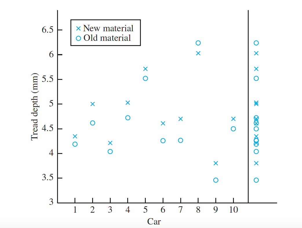
  • let $(X_1, Y_1),…, (X_{10}, Y_{10})$ be the $10$ observed pairs, with $Xi$ representing the tread on the tire made from the new material on the $i^{th}$ car and $Y_i$ representing the tread on the tire made from the old material on the $i^{th}$ car.

  • Let $D_i = X_i − Y_i$ represent the difference between the treads for the tires on the $i^{th}$ car. Let $𝜇_X$ and $𝜇_Y$ represent the population means for $X$ and $Y$, respectively.We wish to find

    a $95\%$ confidence interval for the difference $\mu_X − \mu_Y$. Let $\mu_D$ represent the population mean of the differences. Then $\mu_D = \mu_X −\mu_Y $. It follows that a confidence interval for $\mu_D$ will also be a confidence interval for $\mu_X −\mu_Y$.

  • Since the sample $D_1,…, D_{10}$ is a random sample from a population with mean $𝜇_D$, we can use one-sample methods to find confidence intervals for $𝜇_D$.

  • Let $D_1,…, D_n$ be a small random sample $(n ≤ 30)$ of differences of pairs. If the population of differences is approximately normal, then a level $100(1 − 𝛼)\%$ confidence interval for the mean difference $𝜇_D$ is given by $D \pm t_{n−1,\frac{\alpha}{2}} \frac{s_{D}} {\sqrt{n}}$

    where $s_{D}$ is the sample standard deviation of $D_1,\ldots, D_n$. Note that this interval is the same as given by expression of. If the sample size is large, a level $100(1 − 𝛼)\%$ confidence interval for the mean difference $𝜇_D$ is given by $D \pm z_{𝛼∕2} \sigma_D $

    In practice $\sigma_D$ is approximated with $\frac{s_D}{\sqrt n}$. Note that this interval is the same as that given by expression of single mean.

  

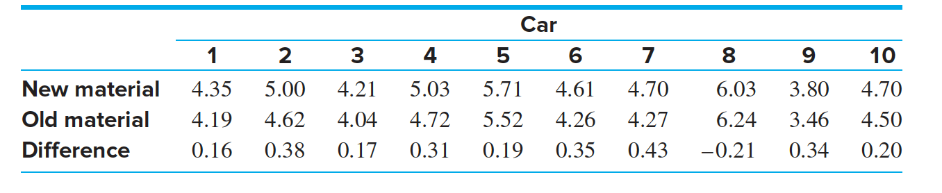
• The Table presents, for each car, the depths of tread for both types of tires as well as the difference between them. We wish to find a $95\% $ confidence interval for the mean difference in tread wear between old and new materials in a way that takes advantage of the reduced variability produced by the paired design.

  • The way to do this is to think of a population of pairs of values, in which each pair consists of measurements from an old type tire and a new type tire on the same car.

  • For each pair in the population, there is a difference (New − Old); thus there is a population of differences.

  • The data are then a random sample from the population of pairs, and their differences are a random sample from the population of differences.

  • Since the sample $D_1,…, D_{10}$ is a random sample from a population with mean $\mu_ D$, we can use one-sample methods to find confidence intervals for $𝜇_D$. In this example, since the sample size is small, we use the Student’s t method.

    The observed values of the sample mean and sample standard deviation are

    ​ $D = 0.232 ~ ~ s_D = 0.183$

    • The sample size is $10$, so there are nine degrees of freedom. The appropriate t value

    ​ is $t_{9,.025} = 2.262$. The confidence interval is therefore $0.232 \pm (2.262)(0.183)∕ \sqrt 10$ , or $(0.101, 0.363)$.

    • When the number of pairs is large, the large-sample methods can be used.