This post covers Introduction to probability from Statistics for Engineers and Scientists by William Navidi.

Basic Ideas

• Random Variables

  • If $X$ is a random variable, and $a$ and $b$ are constants, then

    ​ $ \mu_{aX+b} = a\mu_X + b $

    ​ $𝜎^2_{aX+b}= a𝜎^2_X$

  • If $X$ and $Y$ are random variables, and $a$ and $b$ are constants, then

    ​ $ \mu_{aX+bY} = 𝜇_{aX} + 𝜇_{bY} = a \mu_X + b \mu_Y$

    • let $X$ be the number of parts produced on a given day by machine $A$, and let $Y$ be the number of parts produced on the same day by machine $B$. The total number of parts is $X + Y$, and we have that $ \mu_{X+Y} = \mu_X + \mu_Y$.

  • Variances of Linear Combinations of Independent Random Variables

    If $ X_1, X_2,\ldots, X_n $ are independent random variables, then the variance of the

    ​ sum $ X_1 + X_2 + \ldots + X_n $ is given by \(\sigma^2_{X_1+ X_2+ \ldots + X_n} = \sigma^2_{X_1} + \sigma^2_{X_2} + \ldots + \sigma^2_{X_n} \\\)

• Jointly Distributed Random Variables - We have said that observing a value of a random variable is like sampling a value from a population. In some cases, the items in the population may each have several random variables associated with them. When two or more random variables are associated with each item in a population, the random variables are said to be jointly distributed. For example, imagine choosing a student at random from a list of all the students registered at a university and measuring that student’s height and weight.

  • If $X$ and $Y$ are jointly discrete random variables:

    

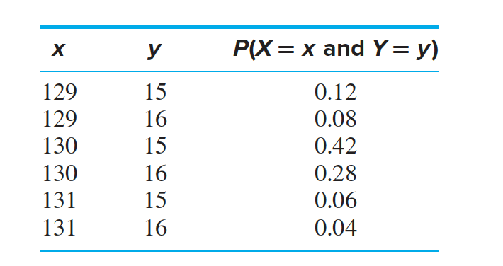
  • The joint probability mass function of $X$ and $Y$ is the function
    \(p(x,y) = P(X = x ~ and ~ Y = y)\\\)

  • The marginal probability mass functions of $X$ and of $Y$ can be obtained from the joint probability mass function as follows:

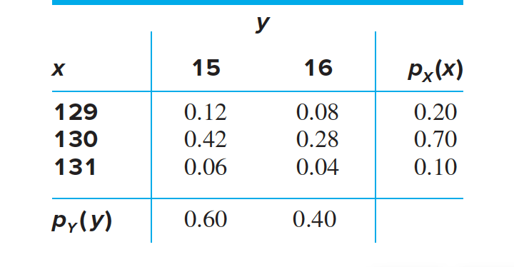
    \[p_X(x) = P(X = x) = \sum_{y} p(x,y)\\ p_Y(y)= P(Y = y) = \sum _x p(x,y)\\\]

  ​ where the sums are taken over all the possible values of $Y$ and of $X$, respectively.

  • The joint probability mass function has the property that
  \[\Sigma_x \Sigma_y p(x,y) = 1 \\\]

  ​ where the sum is taken over all the possible values of $X$ and $Y$.

  

  • Find the probability that a CD cover has a length of 129 mm.

  • Find the probability that a CD cover has a width of 16 mm.

  • Let X and Y be jointly discrete random variables, with joint probability mass function $p(x,y)$. Let $p_X(x)$ denote the marginal probability mass function of $X$ and let $x$ be any number for which $p_X(x) > 0$.

    The conditional probability mass function of $Y$ given $X = x$ is

    ​ $p_{Y \mid X}(y \mid x) = \frac {p(x,y)}{p_X(x)}$

    Note that for any particular values of $x$ and $y$, the value of $p_{Y \mid X}( y \mid x)$ is just the conditional probability $P(Y = y \mid X = x)$.

    • Compute the conditional probability mass function $p_{Y\mid X}(y \mid 130)$.

      $p_{Y \mid X}(15 \mid 130) = P(Y = 15 \mid X = 130)$

      $= \frac{P(Y = 15 ~ and ~X = 130)}{P(X = 130)}$

      $= \frac {0.42}{0.70}$

      $= 0.60$

  • Two random variables X and Y are independent, provided that

    • If X and Y are jointly discrete, the joint probability mass function is equal to the product of the marginals:

    ​ $p(x,y) = p_X(x)p_Y (y)$

    • If $X$ and $Y$ are independent random variables, then

      • If $X$ and $Y$ are jointly discrete, and x is a value for which $p_X(x) > 0$, then

      ​ $ p_{Y \mid X}(y \mid x) = p_Y (y)$

      • The joint probability mass function of the length X and thickness Y of a CD tray cover is given. Are X and Y independent?

      • We must check to see if $P(X = x ~ and ~ Y = y) = P(X = x)P(Y = y)$ for every value of $x$ and $y$. We begin by checking $x = 129, y = 15$:

        $P(X = 129 ~ and ~ Y = 15) = 0.12 = (0.20)(0.60) = P(X = 129)P(Y = 15)$

        Continuing in this way, we can verify that $P(X =x ~ and ~ Y =y)=P(X =x)P(Y =y)$ for every value of x and y. Therefore X and Y are independent.

  • When two random variables are not independent, it is useful to have a measure of the strength of the relationship between them. The population covariance is a measure of a certain type of relationship known as a linear relationship. We will usually drop the term “population,” and refer simply to the covariance.

    • Let $X$ and $Y$ be random variables with means $ \mu_X $ and $ \mu_Y$. The covariance of $X$ and $Y$ is

      \[\begin{align*} Cov(X,Y) &= \mu_{(X−\mu_X)(Y−\mu_Y )}\\ &= \mu_{XY} − \mu_X \mu_Y \end{align*}\]

    

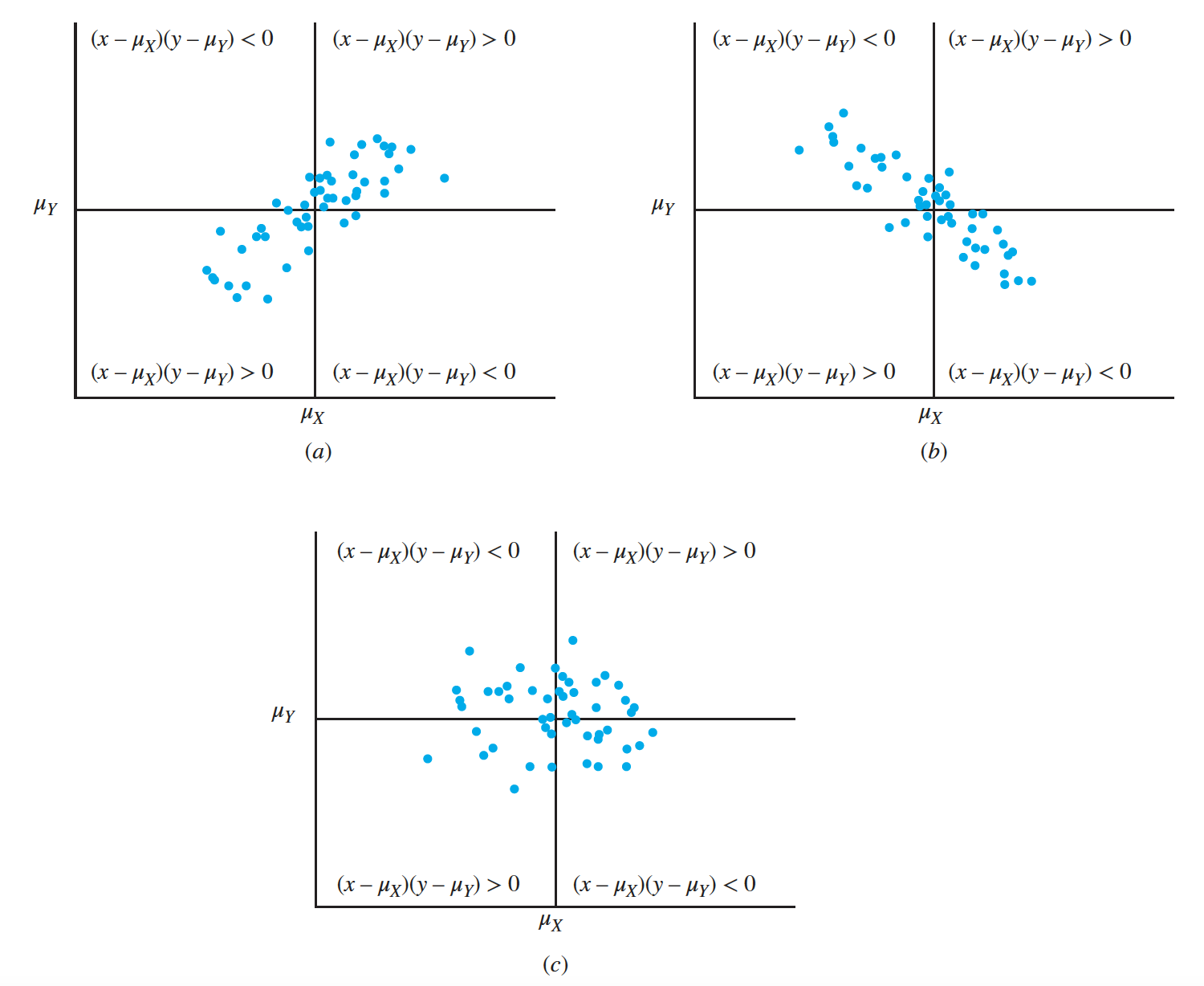
    • If a Cartesian coordinate system is constructed with the origin at $(\mu_X, \mu_Y )$, this product will be positive in the first and third quadrants, and negative in the second and fourth quadrants. It follows that if $Cov(X,Y)$ is strongly positive, then values of $(X,Y)$ in the first and third quadrants will be observed much more often than values in the second and fourth quadrants

    • Finally, if $Cov(X,Y)$ is near $0$, there would be little tendency for larger values of $X$ to be paired with either larger or smaller values of $Y$

    • Find the covariance of X and Y.

      

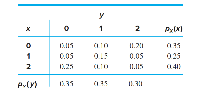
    • We will use the formula $Cov(X,Y) = \mu_{XY} − \mu_X\mu_Y$. First we compute $\mu_{XY}$: \(\mu_{XY} = \sum^2_{x=0} \sum^2_{y=0}xy p(x,y)\) $= (1)(1)(0.15) + (1)(2)(0.05) + (2)(1)(0.10) + (2)(2)(0.05)$

      $= 0.65$ (omitting terms equal to 0)

    • This is a serious drawback in practice, because one cannot use the covariance to determine which of two pairs of random variables is more strongly related, since the two covariances will have different units. What is needed is a measure of the strength of a linear relationship that is unit less. The population correlation is such a measure.

    • Specifically, to compute the correlation between X and Y, one first computes the covariance, and then gets rid of the units by dividing by the product of the standard deviations of X and Y.

  • Correlation Let $X$ and $Y$ be jointly distributed random variables with standard deviations $\sigma_X$ and $ \sigma_Y$. The correlation between $X$ and $Y$ is denoted $ \rho_{X,Y}$ and is given by

    ​ $ \rho_{X,Y} = \frac{Cov(X,Y) }{\sigma_X \sigma_Y}$

    • For any two random variables $X$ and $Y$:

      ​ $−1 ≤ \rho _{X,Y} ≤ 1$

    • we computed $Cov(X,Y) = −0.3475$, $ \mu_X = 1.05$, and $ \mu_Y = 0.95$.We now must compute $ \sigma_X $ and $ \sigma_Y$ . To do this we use the marginal densities of $X$ and of $Y$, we obtain

      \(\sigma^2_{X}= \sum^2_{x=0}x^2p_X(x) − \mu^2_{X}\) $= (02)(0.35) + (12)(0.25) + (22)(0.40) − 1.052$

      $= 0.7475$ \(𝜎^2_Y = \sum^2_{y=0}y^2p_Y (y) − 𝜇^2_Y\\\) $= (02)(0.35) + (12)(0.35) + (22)(0.30) − 0.952$

      $= 0.6475$

      It follows that

      $ \rho_{X,Y} = \frac{−0.3475 }{\sqrt {(0.7475)(0.6475)}}$

      ​ $ = −0.499$

  • Covariance, Correlation, and Independence- If $Cov(X,Y) = \rho_{X,Y} = 0$, then $X$ and $Y$ are said to be uncorrelated.

    • If X and Y are independent, then $X$ and $Y$ are uncorrelated.

    • It is mathematically possible for $X$ and $Y$​ to be uncorrelated without being independent. This rarely occurs in practice.If X and Y are random variables, then \(\sigma^2_{X+Y} = \sigma^2_{X}+ \sigma^2_{Y} + 2 Cov(X,Y)\\ \sigma^2_{X−Y} = \sigma^2_X+ \sigma^2_Y − 2 Cov(X,Y)\\\)

    • If $X$ and $Y$ are independent random variables with variances $𝜎^2_X$ and $𝜎^2_Y$ , then the variance of the sum $X + Y$ is \(𝜎^2_{X+Y} = 𝜎^2_X+ 𝜎^2_Y\\\) The variance of the difference $X − Y$ is \(𝜎^2_{X−Y} = 𝜎^2_X+ 𝜎^2_Y\\\)

    • Assume that the mobile computer moves from a random position $(X,Y)$ vertically to the point $(X, 0)$, and then along the x axis to the origin. c means of $X$ and of $Y$ are $𝜇_X = 4∕5 = 0.800$, and $𝜇_Y = 8∕15 = 0.533$. The variances $ \sigma^2X= 0.02667$ and $ \sigma^2{Y} = 0.04889$. Find the mean and variance of the distance traveled.

  • The items in a simple random sample may be treated as independent, except when the sample is a large proportion (more than $5\%$) of a finite population. From here on, unless explicitly stated to the contrary, we will assume this exception has not occurred, so that the values in a simple random sample may be treated as independent random variables.

  • if $X_1, \ldots , X_n$ is a simple random sample from a population with mean $\mu$ and variance $\sigma^2$, then the sample mean $X$ is the linear combination

    $X = \frac{1}{n}X_1 + \ldots + \frac{1}{n}X_n$

  • From this fact we can compute the mean and variance of $X$.

    $\mu_{\overline X} = \mu_{\frac{1}{n}X_1+\ldots+\frac{1}{n}X_n}$

    $ = \frac{1}{n}\mu_{X_1} + \ldots + \frac{1}{n}\mu_{X_n}$

    $= \frac{1}{n}\mu +\ldots+ \frac{1}{n}\mu$

    $= (n)\frac{1}{n}\mu$

    $ = \mu$

  • The items in a simple random sample may be treated as independent random variables. Therefore

    \[\begin{align*} \sigma^2_{\overline X} &= \sigma^2_{\frac{1}{n}X_1+ \ldots +\frac{1}{n}X_n} \\ &= \frac{1}{n^2}\sigma^2_{X_1} + \ldots + \frac{1}{n^2}\sigma^2_{X_n} \\ &= \frac{1}{n^2}\sigma^2 +\ldots+ \frac{1}{n^2}\sigma^2 \\ &= \frac{1}{n^2}\sigma^2 +\ldots+ \frac{1}{n^2}\sigma^2 \\ &= (n)\frac{1}{n^2}\sigma^2 \\ &= \frac{\sigma^2}{n} \end{align*}\]

• A piston is placed inside a cylinder. The clearance is the distance between the edge of the piston and the wall of the cylinder and is equal to one-half the difference between the cylinder diameter and the piston diameter. Assume the piston diameter has a mean of $80.85$ cm with a standard deviation of $0.02$ cm. Assume the cylinder diameter has a mean of $80.95$ cm with a standard deviation of $0.03$ cm. Find the mean clearance. Assuming that the piston and cylinder are chosen independently, find the standard deviation of the clearance.