This post covers Introduction to probability from Statistics for Engineers and Scientists by William Navidi.

Basic Ideas

• Normal approximation to Binomial &​ other probability densities

  • The Central Limit Theorem

    • The Central Limit Theorem is by far the most important result in statistics

    • if we draw a large enough sample from a population, then the distribution of the sample mean is approximately normal, no matter what population the sample

      was drawn from.

    • This allows us to compute probabilities for sample means using the z table, even though the population from which the sample was drawn is not normal.We now explain this more fully.

    • If one could draw every possible sample of size $n$ from the original population, and compute the sample mean for each one, the resulting collection would be the population of sample means.

    • Let $X_1, \ldots, X_n$ be a simple random sample from a population with mean $\mu$ and variance $\sigma^{2}$. Let $\overline{X} = X_{1} +\ldots+ X_{n}$ be the sample mean. Let $S_{n} = X_{1} + \ldots + X_{n}$ be the sum of the sample observations. Then if $n$ is sufficiently large,

      $ \overline{X} ∼ N$$(\mu, \frac{\sigma^{2}}{n})$ approximately and

      $S_n \sim N(n\mu, n\sigma^{2})$ approximately

    • The sum of the sample items is equal to the mean multiplied by the sample size, that is, $S_{n} = n_{X}$

    • The Central Limit Theorem says that $X$ and $S_{n}$ are approximately normally distributed, if the sample size $n$ is large enough. For most populations, if the sample size is greater than $30$, the Central Limit Theorem approximation is good.

    • The natural question to ask is: How large is large enough? The answer depends on the shape of the underlying population

    • If the sample is drawn from a nearly symmetric distribution, the normal approximation can be good even for a fairly small value of $n$. However, if the population is heavily skewed, a fairly large $n$ may be necessary.

    • Empirical evidence suggests that for most populations, a sample size of $30$ or more is large enough for the normal approximation to be adequate

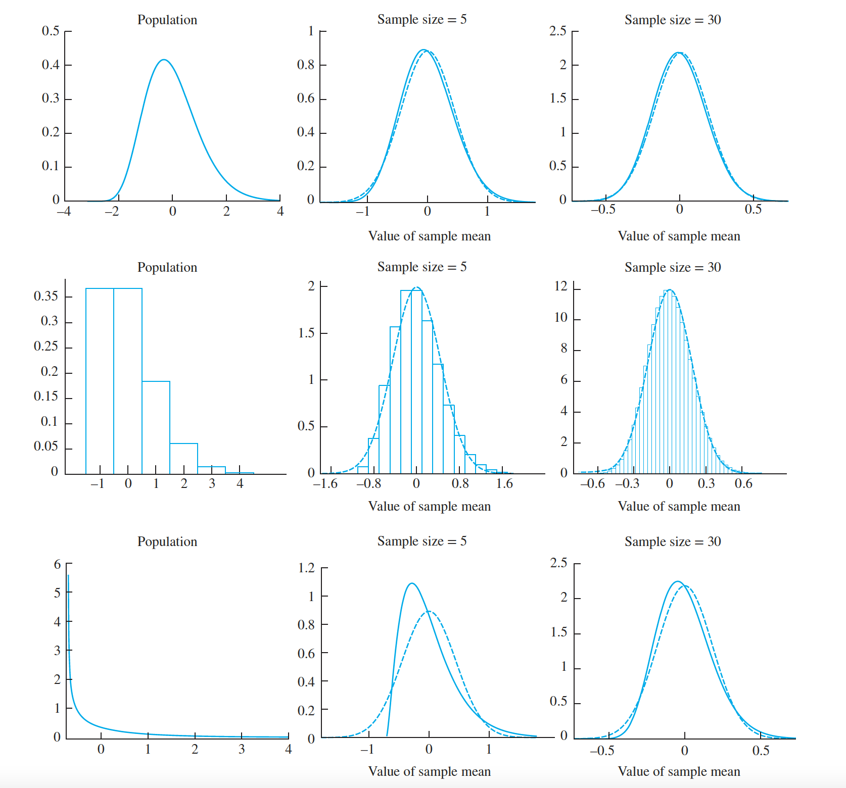
• Middle row: The original distribution is somewhat skewed. Even so, the normal approximation is reasonably close even for a sample of size $5$, and very good for a sample of size $30$.
• Top row: Since the original distribution is nearly symmetric, the normal approximation is good even for a sample size as small as $5$.
• Bottom row: The original distribution is highly skewed. The normal approximation is not good for a sample size of $5$, but is reasonably good for a sample of size $30$. Note that two of the original distributions are continuous, and one is discrete. The Central Limit Theorem holds for both continuous and discrete distributions.
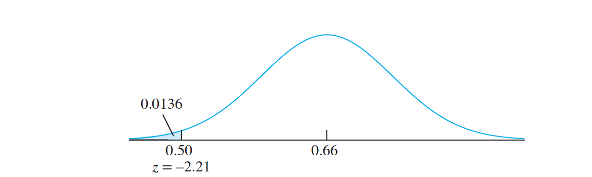
• Let $X$ denote the number of flaws in a 1 in. length of copper wire. The probability mass function of $X$ is presented in the following table. One hundred wires are sampled from this population. The population mean number of flaws is $ \mu = 0.66$, and the population variance is $\sigma^2 = 0.5244$. What is the probability that the average number of flaws per wire in this sample is less than $0.5$?

• Accuracy of the Continuity Correction
  • For binomial distributions with large $n$ and small $p$, however, when computing a probability that corresponds to an area in the tail of the distribution, the continuity correction can in some cases reduce the accuracy of the normal approximation somewhat. This results from the fact that the normal approximation is not perfect; it fails to account for a small degree of skewness in these distributions
• Normal Approximation to the Poisson
  • If $X ∼ Poisson(\lambda)$, then $X$ is approximately binomial with $n$ large and $np =\lambda$. Recall also that $ \mu_X = \lambda $ and $ 𝜎_{2X} = \lambda $.
  • It follows that if $ \lambda $ is sufficiently large, i.e., $\lambda > 10$, then $X$ is approximately binomial, with $np > 10$. It follows from the Central Limit Theorem that $X$ is also approximately normal, with mean and variance both equal to $\lambda$. Thus we can use the normal distribution to approximate the Poisson.
  • The number of hits on a website follows a Poisson distribution, with a mean of $27$ hits per hour. Find the probability that there will be $90$ or more hits in three hours.

• Continuity Correction for the Poisson Distribution
  • Since the Poisson distribution is discrete, the continuity correction can in principle be applied when using the normal approximation.
  • For areas that include the central part of the curve, the continuity correction generally improves the normal approximation, but for areas in the tails the continuity correction sometimes makes the approximation worse.
  • We will not use the continuity correction for the Poisson distribution.