This post covers Introduction to probability from Statistics for Engineers and Scientists by William Navidi.

Cumulative normal distribution (z table)

Basic Ideas

• The Normal Distribution

  • The normal distribution is continuous rather than discrete. The mean of a normal

    random variable may have any value, and the variance may have any positive value.

  • The probability density function of a normal random variable with mean $\mu$ and variance $\sigma$ is given by

    ​ $f (x) = \frac {1}{ \sigma \sqrt 2\pi} e^{−(x−𝜇)^{2}}∕(2𝜎^{2})$

  • If $X$ is a random variable whose probability density function is normal with mean $\mu$ and variance $\sigma^{2}$, we write $ X \sim N(\mu, \sigma^{2})$.

    

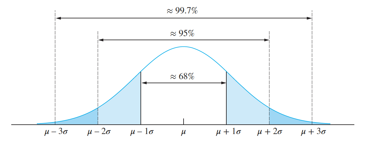
  • Note that the normal curve is symmetric around $\mu$, so that $\mu$ is the median as well as the mean. It is also the case that for any normal population

  • We often convert from the units in which the population items were originally measured to standard units. Standard units tell how many standard deviations an observation is from the population mean. In general, we convert to standard units by subtracting the mean and dividing by the standard deviation. Thus, if $x$ is an item sampled from a normal population with mean $\mu$ and variance $\sigma^{2}$, the standard unit equivalent of $x$ is the number $z$, where

    ​ $z = \frac{x-\mu}{\sigma}$

  • The z-score is an item sampled from a normal population with mean $0$ and standard deviation $1$. This normal population is called the standard normal population.

• Ball bearings manufactured for a certain application have diameters (in mm) that are normally distributed with mean $5$ and standard deviation $0.08$. A particular ball bearing has a diameter of $5.06$ mm. Find the z-score.

• The diameter of a certain ball bearing has a z-score of −1.5. Find the diameter in the original units of mm.

• The proportion of a normal population that lies within a given interval is equal to the area under the normal probability density above that interval

• Interestingly enough, areas under this curve cannot be found by the method, taught in elementary calculus, of finding the antiderivative of the function and plugging in the limits of integration. This is because the antiderivative of this function is an infinite series and cannot be written down exactly. Instead, areas under this curve must be approximated numerically

• Find the area under the normal curve between $z = 0.71$ and $z = 1.28$.

  

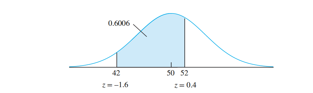
• Lifetimes of batteries in a certain application are normally distributed with mean $50$ hours and standard deviation $5$ hours. Find the probability that a randomly chosen battery lasts between $42$ and $52$ hours.

  

• Estimating the Parameters of a Normal Distribution
• The parameters $\mu$ and $\sigma^{2}$ of a normal distribution represent its mean and variance, respectively. Therefore, if $X_{1},\ldots, X_{n}$ are a random sample from a $N(\mu, \sigma^{2})$ distribution, $\mu$ is estimated with the sample mean $ \overline{X}$ and $𝜎^{2}$ is estimated with the sample variance $s^{2}$. As with any sample mean, the uncertainty in $ \overline{X}$ is $\sigma∕ \sqrt{n}$, which we replace with $\frac{s}{\sqrt{n}}$ if $\sigma$ is unknown. In addition $\mu_\overline{X} = \mu $, so is unbiased for $\sigma$.
• A chemist measures the temperature of a solution in $\deg C$. The measurement is denoted $C$, and is normally distributed with mean $40^0 C$ and standard deviation $1^0 C$. The measurement is converted to $deg ~ F$ by the equation $F = 1.8C + 32$. What is the distribution of $F$?

• Linear Functions of Normal Random Variables

  • Let $X \sim N(𝜇, 𝜎^{2})$, and let $a \neq 0$ and $b$ be constants. Then $aX + b \sim N(a\mu + b, a^{2} 𝜎^{2})$

• Linear Combinations of Independent Normal Random Variables

  • Let $X_{1}, X{2},\ldots, X_{n}$ be independent and normally distributed with means

    $\mu{1}, \mu{2},…, \mu_{n}$ and variances $ \sigma_{1}^{2}, \sigma_{1}^{2}, \ldots, \sigma_{1}^{2} $. Let $ c_{1}, c_{2}, \ldots , c_{n} $ be constants, and

    $c_{1}X_{1} + c_{2}X_{2} +⋯+ c_{n}X_{n}$ be a linear combination. Then

    $c_1 X_1+ c_2 X_2+ \ldots c_n X_n \sim N(c_1 \mu_1 + c_2 \mu_2 + \ldots + c_n \mu_n, c_1^2 \sigma_1^2 + c_2^2 \sigma_1^2 + \ldots + c_n^2 \sigma_n^2 )$

• In the article “Advances in Oxygen Equivalent Equations for Predicting the Properties of Titanium Welds” the authors propose an oxygen equivalence equation to predict the strength, ductility, and hardness of welds made from nearly pure titanium. The equation is $E = 2C+3.5N+O$, where $E$ is the oxygen equivalence, and $C, N, and ~ O $ are the proportions by weight, in parts per million, of carbon, nitrogen, and oxygen, respectively (a constant term involving iron content has been omitted). Assume that for a particular grade of commercially pure titanium, the quantities $C$, $N$, and $O$ are approximately independent and normally distributed with means

  ​ $\mu_C = 150, \mu_N =200, \mu_O = 1500$, and standard deviations

  ​ $ \sigma_C = 30, \sigma_N = 60, \sigma_O = 100$.

  Find the distribution of $E$. Find $P(E > 3000)$.

• If $X_1,\ldots , X_n$ is a random sample from any population with mean $\mu$ and variance $\sigma^2$

  , then the sample mean $\overline X$ has mean $\mu_\overline X = \mu$ and variance $\sigma^2_\overline X= \sigma^2∕n$.

  If the population is normal, then $X$ is normal as well, because it is a linear combination of $X_1,…, X_n$ with coefficients $c_1 = \ldots c_n = 1∕n$.

• How Can I Tell Whether My Data Come from a Normal Population?

  • Large samples from normal populations have histograms that look something like the normal density function—peaked in the center, and decreasing more or less symmetrically on either side.

  • when the sample size is small. Unfortunately, for small data sets that do not contain outliers, it is difficult to determine whether the population is approximately normal.