This post covers Introduction to probability from Statistics for Engineers and Scientists by William Navidi.

Upper percentage points for the Student’s t distribution

Basic Ideas

• Small-Sample Confidence Intervals for a Population Mean

  • If $ \overline X $ is the mean of a large sample of size $n$ from a population with mean $\mu$ and variance $\sigma^2$, then the Central Limit Theorem specifies that $ \overline X ∼ N(\mu,\frac{\sigma^2}{ n})$.

  • The quantity $ \frac {(\overline X −𝜇)}{(\frac{\sigma} {\sqrt n})}$ then has a normal distribution with mean $0$ and variance $1$.

  • In addition, the sample standard deviation s will almost certainly be close to the population standard deviation $\sigma$.

  • For this reason the quantity $ \frac {(\overline X −𝜇)}{(\frac{s} {\sqrt n})}$ is approximately normal with mean 0 and variance 1, so we can look up probabilities pertaining to this quantity in the standard normal table $(z ~ table)$. This enables us to compute confidence intervals of various levels for the population mean $\mu$.

  • The Student’s t distribution

    • What can we do if $\overline X$ is the mean of a small sample?
      • If the sample size is small, $s$ may not be close to $\sigma$, and $\overline X $ may not be approximately normal.
      • If we know nothing about the population from which the small sample was drawn, there are no easy methods for computing confidence intervals.
      • However, if the population is approximately normal, $\overline X $ will be approximately normal even when the sample size is small. It turns out that we can still use the quantity ,$ \frac {(\overline X −𝜇)}{(\frac{s} {\sqrt n})}$ but since $s$ is not necessarily close to $\sigma$, this quantity will not have a normal distribution.
      • It has the Student’s t distribution with $n−1$ degrees of freedom, which we denote $t_{(n−1)}$.
    • Don’t Use the Student’s t Statistic If the Sample Contains Outliers

  • Confidence Intervals Using the Student’s t distribution

    • The Student’s t distribution was discovered in 1908 by William Sealy Gossett

    • Let $X_1, \ldots , X_n$ be a small (e.g., $n < 30$) sample from a normal population with

      mean $ \mu $. Then the quantity$ \frac {(\overline X −𝜇)}{(\frac{s} {\sqrt n})}$ has a Student’s t distribution with $n − 1$ degrees of freedom, denoted $t_{(n−1)}$.

    • When n is large, the distribution of the quantity $ \frac {(\overline X −𝜇)}{(\frac{s} {\sqrt n})}$ is very close to normal, so the normal curve can be used, rather than the Student’s t.

      

    • Plots of the probability density function of the Student’s t curve for various

    ​ degrees of freedom.

    • The normal curve with mean 0 and variance 1 (z curve) is plotted for comparison.
    • The t curves are more spread out than the normal, but the amount of extra spread decreases as the number of degrees of freedom increases.
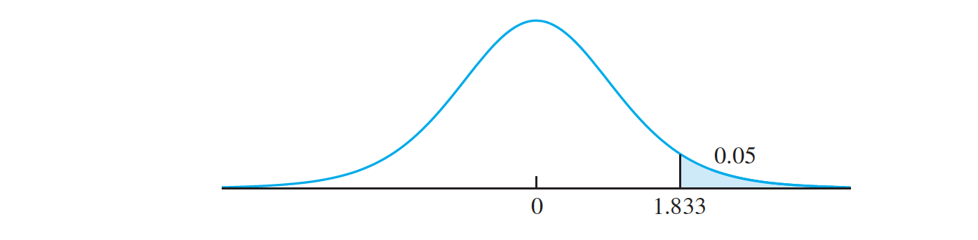
    • A random sample of size 10 is to be drawn from a normal distribution with mean 4. The Student’s t statistic t = $ \frac {(\overline X −4)}{(\frac{s} {\sqrt 10})}$ is to be computed. What is the probability that $t > 1.833$?

• Don’t Use the Student’s t Statistic If the Sample Contains Outliers

  • Confidence Intervals Using the Student’s t distribution

    • When the sample size is small, and the population is approximately normal, we can use the Student’s t distribution to compute confidence intervals.

    • The confidence interval in this situation is constructed, the z-score is replaced with a value from the Student’s t distribution.

    • The quantity $ \frac {(\overline X −𝜇)}{(\frac{s} {\sqrt n})}$ has a Student’s t distribution with $n − 1$ degrees of freedom

    • To produce a level $100(1 − 𝛼)\%$ confidence interval, let $t_{n−1,\alpha∕2}$ be the $1− \frac{\alpha}{2}$ quantile of the Student’s t distribution with $n−1$​ degrees of freedom, that is, the value which cuts off an area of $\frac{ \alpha}{2}$ in the right-hand tail.

    • Then a level 100(1 − 𝛼)% confidence interval for the population

      mean $𝜇$ is $ \overline X − t_{n−1,𝛼∕2}(\frac{s} {\sqrt n}) < 𝜇 < \overline X + t_{n−1,𝛼∕2}(\frac{s} {\sqrt n}), or \overline X \pm t_{n−1,𝛼∕2}(\frac{s} {\sqrt n})$.

• How to determine whether the Student’s t distribution is appropriate?

  • The Student’s t distribution is appropriate whenever the sample comes from a population that is approximately normal.

  • In many cases, however, one must decide whether a population is approximately normal by examining the sample.

  • when the sample size is small, departures from normality may be hard to detect.

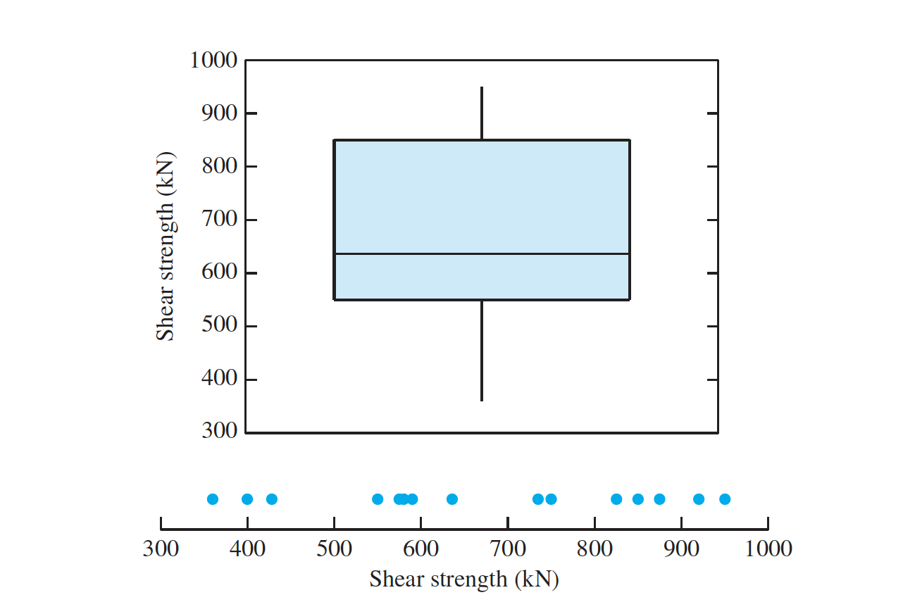
  • The measurements of the nominal shear strength (in kN) for a sample of $15$ prestressed

    concrete beams. The results are

    $580 ~ 400 ~ 428 ~ 825 ~ 850 ~ 875 ~ 920 ~ 550 ~ 575 ~ 750 ~ 636 ~ 360 ~ 590 ~ 735 ~ 950$

    Is it appropriate to use the Student’s t statistic to construct a $99\%$ confidence interval for the mean shear strength? If so, construct the confidence interval. If not, explain why not.

• Use z, Not t, if $\sigma$ is Known

  • Occasionally a small sample may be taken from a normal population whose standard deviation $\sigma$ is known. In these cases, we do not use the Student’s t curve, because we are not approximating $\sigma$ with $s$.

  • Let $X_1,\ldots, X_n$ be a random sample (of any size) from a normal population with mean $\mu$. If the standard deviation $ \sigma$ is known, then a level $100(1−𝛼)\%$ confidence

    interval for 𝜇 is $ \overline X \pm z_{𝛼∕2} \frac {\sigma} {\sqrt n} $

  • Let $ \overline X$ be a single value sampled from a normal population with mean $ \mu $. If the

    standard deviation $\sigma$ is known, then a level $100(1 − 𝛼)\%$ confidence interval for

    $\mu$ is $ \overline X \pm z_{𝛼∕2} {\sigma} $