This post covers Introduction to probability from Statistics for Engineers and Scientists by William Navidi.

Basic Ideas

• Statistics

  • Statistics is the field of study concerned with the collection, analysis, and interpretation of uncertain data. The methods of statistics allow scientists and engineers to design valid experiments and to draw reliable conclusions from the data they produce.
  • The applications of statistics to science and engineering, it is worth mentioning that the analysis and interpretation of data are playing an important role.
  • The basic idea behind all statistical methods of data analysis is to make inferences about a population by studying a relatively small sample chosen from it.

• Consider a machine that makes steel rods for use in optical storage devices. The specification for the diameter of the rods is $0.45\pm 0.02$ cm. During the last hour, the machine has made $1000$ rods. The quality engineer wants to know approximately how many of these rods meet the specification. He does not have time to measure all $1000$ rods. So he draws a random sample of $50$ rods, measures them, and finds that $46$ of them ($92\%$) meet the diameter specification. Now, it is unlikely that the sample of $50$ rods represents the population of $1000$ perfectly. The proportion of good rods in the population is likely to differ somewhat from the sample proportion of $92\%$. What the engineer needs to know is just how large that difference is likely to be. For example, is it plausible that the population percentage could be as high as $95\%? 98\%?$ As low as $90\%? 85\%?$

• Here are some specific questions that the engineer might need to answer on the basis of these sample data:

  • The engineer needs to compute a rough estimate of the likely size of the difference between the sample proportion and the population proportion. How large is a typical difference for this kind of sample?
  • The quality engineer needs to note in a logbook the percentage of acceptable rods manufactured in the last hour. Having observed that 92% of the sample rods were good, he will indicate the percentage of acceptable rods in the population as an interval of the form $92\%° \pm x\%$, where $x$ is a number calculated to provide reasonable certainty that the true population percentage is in the interval. How should $x$ be calculated?
  • The engineer wants to be fairly certain that the percentage of good rods is at least $90\%$; otherwise he will shut down the process for recalibration. How certain can he be that at least $90%$ of the $1000$ rods are good?

• Computation of a standard deviation, construction of a confidence interval, hypothesis test

• Inferential statistics- drawing conclusions from data

• Descriptive statistics- methods of collecting data

• A population is the entire collection of objects or outcomes about which information is sought.

• A sample is a subset of a population, containing the objects or outcomes that are actually observed.

• A simple random sample of size $n$ is a sample chosen by a method in which each collection of $n$ population items is equally likely to make up the sample, just as in a lottery.

• The items in a sample are independent if knowing the values of some of the items does not help to predict the values of the others.

• Items in a simple random sample may be treated as independent in many cases encountered in practice. The exception occurs when the population is finite and the sample consists of a substantial fraction (more than 5%) of the population.

• The Sample Mean - Let $X_{1},…, X_{n}$ be a sample. The sample mean is

  ​ $\hat{X} = \frac{1}{n} \Sigma^n_{i=1}X_{i}$​​

  • A simple random sample of five men is chosen from a large population of men, and their heights are measured. The five heights (in inches) are $65.51, 72.30, 68.31, 67.05, ~ and ~ 70.68$​. Find the sample mean.

• Let $ X_{1},…, X_{n}$​​ be a sample. The sample standard deviation is the quantity

  ​ $s = \sqrt{\frac{1}{n − 1}\Sigma^{n} _{i=1}(Xi − \hat{X})^2}$​​​

  • Find the sample variance and the sample standard deviation for the height data

• The Sample Median
  • If $n$​ numbers are ordered from smallest to largest: If $n$​ is odd, the sample median is the number in position $\frac{n + 1}{2}$​. If $n$​ is even, the sample median is the average of the numbers in positions $\frac{n}{2}$​ and $\frac{n+1}{2}$​.
  • Find the sample median for the height data

• The Trimmed Mean

  • the trimmed mean is a measure of center that is designed to be unaffected by outliers. The trimmed mean is computed by arranging the sample values in order, “trimming” an equal number of them from each end, and computing the mean of those remaining. If $p\%$ of the data are trimmed from each end, the resulting trimmed mean is called the “$p\%$ trimmed mean.”

• In the article “Evaluation of Low-Temperature Properties of HMA Mixtures” , the following values of fracture stress (in megapascals) were measured for a sample of 24 mixtures of hot-mixed asphalt (HMA).

  30	75	79	80	80	105	126	138	149	179	179	199
  223	232	232	236	240	242	245	247	254	274	384	470

  Compute the mean, median, and the $5\%$, $10\%,$ and $20\%$ trimmed means.

• Outliers- Sometimes a sample may contain a few points that are much larger or smaller than the rest. Such points are called outliers. Outliers should always be scrutinized, and any outlier that is found to result from an error should be corrected or deleted. Not all outliers are errors. Sometimes a population may contain a few values that are much different from the rest, and the outliers in the sample reflect this fact.
• The Mode and the Range-
  • The sample mode is the most frequently occurring value in a sample.
  • The range is the difference between the largest and smallest values in a sample.
  • Find the modes and the range for the sample

• Quartiles-
  • Quartiles divide it as nearly as possible into quarters.
  • A sample has three quartiles
  • To find the first quartile, compute the value $0.25(n + 1)$.
  • The third quartile is computed in the same way, except that the value $0.75(n+1)$​​.

• Percentiles-
  • Order the sample values from smallest to largest, and then compute the quantity $(p∕100)(n + 1)$​, where $n$​ is the sample size.

• Standard error of the mean- The next quantity (SE Mean) is the standard error of the mean. The standard error of the mean is equal to the standard deviation divided by the square root of the sample size.

• A numerical summary of a sample is called a statistic. A numerical summary of a population is called a parameter. Statistics are often used to estimate parameters.

• Graphical Summaries

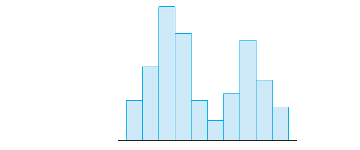
  • A histogram is a graphic that gives an idea of the “shape” of a sample, indicating regions

    where sample points are concentrated and regions where they are sparse

  • To construct a histogram:

    • Choose boundary points for the class intervals.
    • Compute the frequency and relative frequency for each class. (Relative frequency is optional if the classes all have the same width.)
    • Compute the density for each class, according to the formula
    • Density = Relative FrequencyClass Width

  (This step is optional if the classes all have the same width.)

  • Draw a rectangle for each class. If the classes all have the same width, the heights of the rectangles may be set equal to the frequencies, the relative frequencies, or the densities. If the classes do not all have the same width, the heights of the rectangles must be set equal to the densities.

  • it is good to have more intervals rather than fewer, but it is also good to have large numbers of sample points in the intervals

    

  

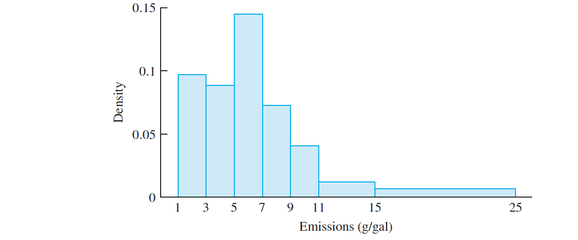
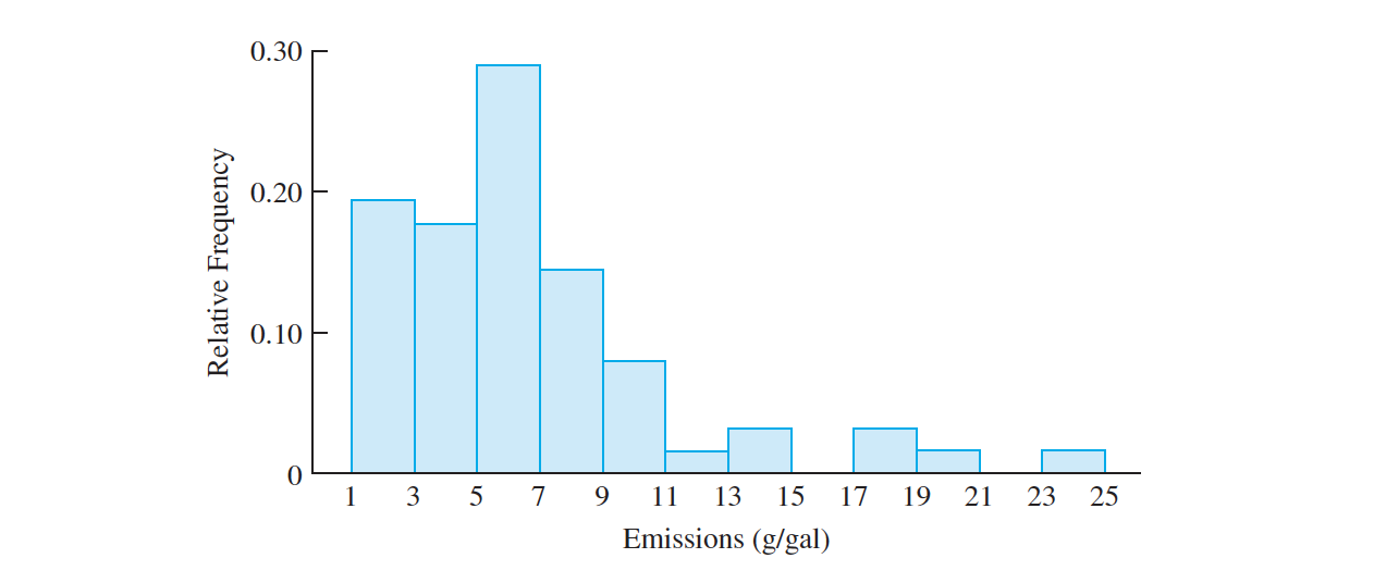
  • Use the histogram with equal intervals to determine the proportion of the vehicles in the sample with emissions between $7$ and $11$ g/gal.

• Use the histogram with unequal intervals to determine the proportion of the vehicles in the sample with emissions between $9$ and $15$ g/gal.

• Forty-five specimens of a certain type of powder were analyzed for sulfur trioxide content. Following are the results, in percent. The list has been sorted into numerical order.

  $14.1 ~ 14.4 ~ 14.7 ~ 14.8 ~ 15.3 ~ 15.6 ~ 16.1 ~ 16.6 ~ 17.3 ~ 14.2 ~ 14.4 ~ 14.7 ~ 14.9 ~ 15.3 ~ 15.7 ~ 16.2 ~ 17.2 ~ 17.3$

  $14.3 ~ 14.4 ~ 14.8 ~ 15.0 ~ 15.4 ~ 15.7 ~ 16.4 ~ 17.2 ~ 17.8 14.3 ~ 14.4 ~ 14.8 ~ 15.0 ~ 15.4 ~ 15.9 ~ 16.4 ~ 17.2 ~ 21.9$

  $14.3 ~ 14.6 ~ 14.8 ~ 15.2 ~ 15.5 ~ 15.9 ~ 16.5 ~ 17.2 ~ 22.4$

  • Construct a histogram for these data

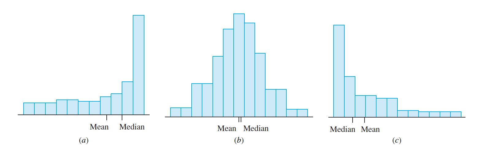
• The mean is near the center of mass of the histogram, that is, it is near the point where the histogram would balance if supported there.
• For a histogram skewed to the right, more than half the data will be to the left of the center of mass.

​

• Unimodal and Bimodal Histograms

  • A histogram is unimodal if it has only one peak, or mode, and bimodal if it has two clearly distinct modes

  

• The histograms for the durations following short or long eruptions are both unimodal, and their modes form the two modes of the histogram for the full sample.

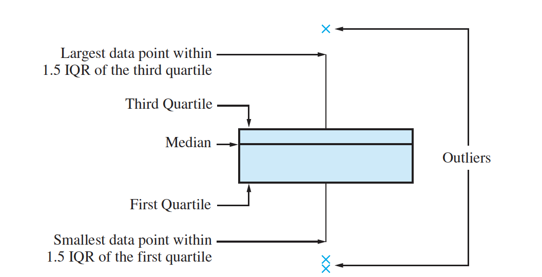
• Boxplots- A boxplot is a graphic that presents the median, the first and third quartiles, and any outliers that are present in a sample.

• It can be used to determine the regions in which the sample values are more densely crowded and the regions in which they are more sparse.

  

• Construct a boxplot for sulfur trioxide content. Does the boxplot show any outliers?

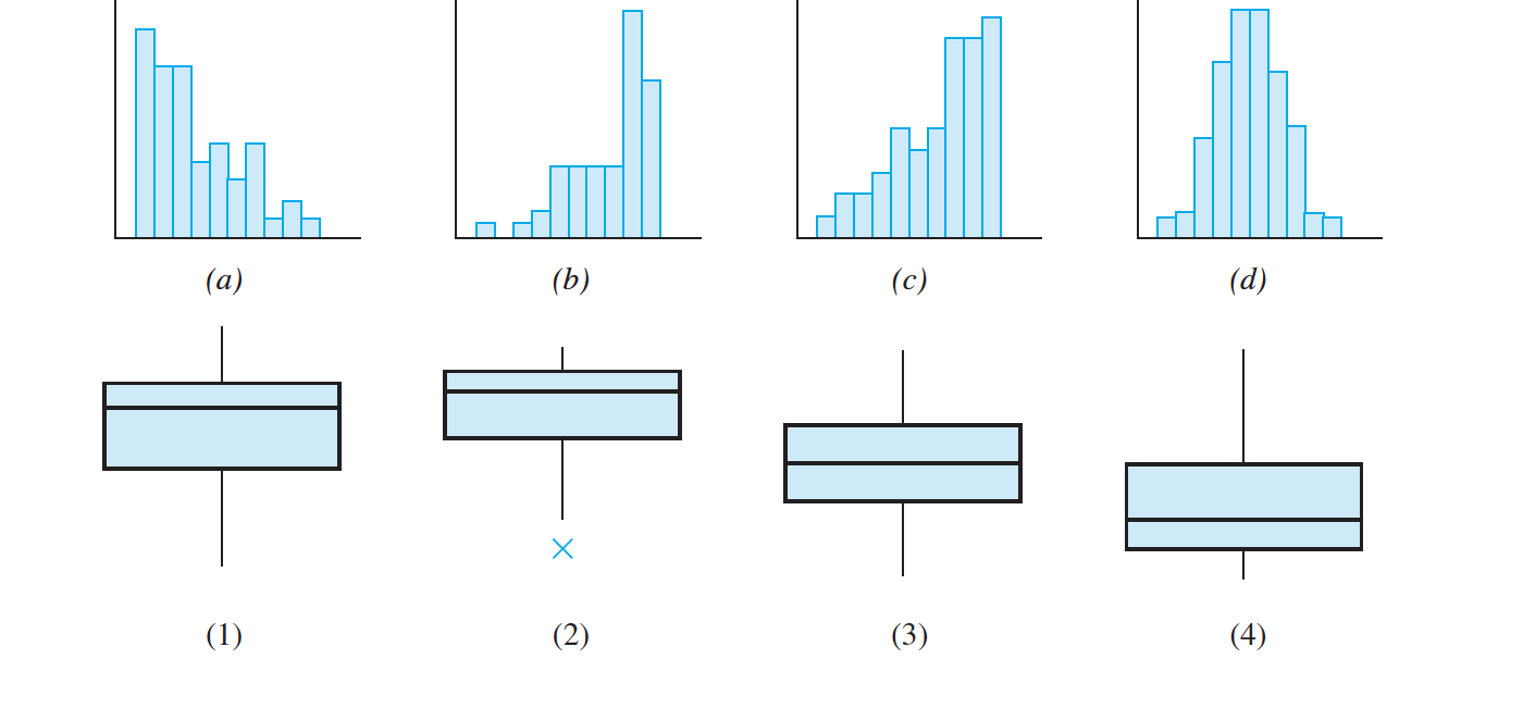
• Match each histogram to the boxplot that represents the same data set.