The Least-Square estimation
Published:
This post covers Introduction to probability from Statistics for Engineers and Scientists by William Navidi.
Basic Ideas
The Least-Square estimation
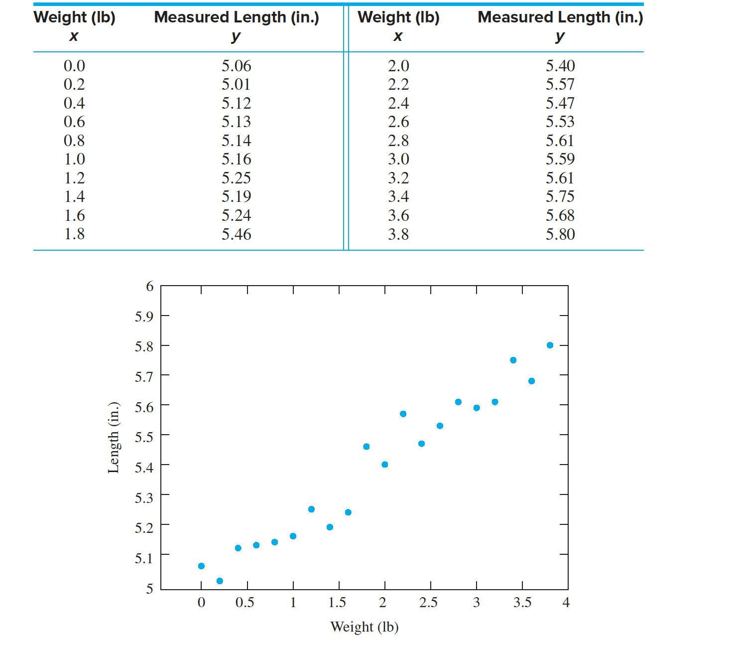
- Figure presents the scatterplot of y versus x with the least-squares line superimposed.
- We wish to use these data to estimate the spring constant $\beta_1$ and the unloaded length $ \beta_0$.
- We write the equation of the line as
- The quantities: $\beta_0$ and $\beta_1$ are called the least-squares coefficients. The coefficient $ \hat \beta_0$, the slope of the least-squares line, is an estimate of the true spring constant $ \beta_0$, and the coefficient $\hat \beta_1$, the intercept of the least-squares line, is an estimate of the true unloaded length $ \beta_1$.

- Points above the least-squares line have positive residuals, and points below the least-squares line have negative residuals
- We now define what we mean by “best.” For each data point $(x_i, y_i)$, the vertical distance to the point $(x_i, \hat y_i)$ on the least-squares line is $e_i = y_i- \hat y_i$
- We define the least-squares line to be the line for which the sum of the squared residuals $ \Sigma^n_{i =1} e^2_i$ is minimized. In this sense, the least-squares line fits the data better than any other line.
- With only one independent variable, are known as simple linear regression models. Linear models with more than one independent variable are called multiple regression models.
Computing the Equation of the Least-Squares Line

To compute the equation of the least-squares line, we must determine the values for the slope $ \hat \beta_1$ and the intercept $ \hat \beta_0$ that minimize the sum of the squared residuals $\Sigma^n_{i=1} e^2_i$ \(\begin{align*} e_i = y_i- \hat y_i = y_i − \hat \beta_0 − \hat \beta_1 x_i\\ \end{align*}\) To do this, we first express $e_i$ in terms of ̂ $ \hat \beta_0$ and $ \hat \beta_1$:
Therefore $ \hat \beta_0$ and $ \hat \beta_1$ are the quantities that minimize the sum
\[\begin{align*} S = \Sigma_{i=1}^ne^2_i= \Sigma_{i=1}^n(y_i − \hat \beta_0 − \hat \beta_1 x_i)^2\\ \end{align*}\]These quantities are
\[\hat \beta_1 = \frac{\Sigma^n_{i=1}(x_i − \overline x)(y_i − \overline y)}{ \Sigma^n_{i=1}(x_i − \overline x)^2}\\\] \[\hat \beta_0 = y − \hat \beta_1x \\\]The quantity $ \hat y_i = \hat \beta_0+ \hat \beta_1 x_i$ is called the fitted value, and the quantity $e_i$ is called the residual associated with the point $(x_i, y_i)$.
The residual $e_i$ is the difference between the value $y_i$ observed in the data and the fitted value $ \hat y_i$ predicted by the least-squares line.
Derivation of the Least-Squares Coefficients $ \hat \beta_0$ and $ \hat \beta_1$
The least-squares coefficients $ \hat \beta_0$ and $ \hat \beta_1$ are the quantities that minimize the sum
\[\begin{align*} S = \Sigma_{i=1}^ne^2_i= \Sigma_{i=1}^n(y_i − \hat \beta_0 − \hat \beta_1 x_i)^2\\ \end{align*}\]We compute these values by taking partial derivatives of $S$ with respect to $ \hat \beta_0$ and $ \hat \beta_1$ and setting them equal to 0. Thus $ \hat \beta_0$ and $ \hat \beta_1$ are the quantities that solve the simultaneous equations
\[\frac {\delta S} { \delta \hat \beta_0} = − \Sigma^n_{i=1} 2(y_i − \hat \beta_0 − ̂ \beta_1x_i) = 0\] \[\frac {\delta S} { \delta \hat \beta_1} = − \Sigma^n_{i=1} 2x_i(y_i − \hat \beta_0 − ̂ \beta_1x_i) = 0\]These equations can be written as a system of two linear equations in two unknowns:
\[n \hat \beta_0 + ( \Sigma^n_{i=1} x_i) \hat \beta_1 = \Sigma^n_{i=1} y_i\] \[( \Sigma^n_{i=1}x_i) \hat \beta_0 +( \Sigma^n_{i=1}x^2_i) \hat \beta_1 = \Sigma^n_{i=1}x_iy_i\]We solve Equation for $ \hat \beta_0$, we obtain
\[\hat\beta_0 =\Sigma^n_{i=1} \frac{y_i}{n}−\hat\beta _1\Sigma^n_{i=1}\frac{x_i}{n}\]Now substitute $y − \hat \beta_1x$ for $ \hat \beta_0$ in to obtain $\hat \beta_1$
\((\Sigma^n_{i=1} x_i)(y − \hat \beta_1x) +( \Sigma^n_{i=1}x^2_i) \beta_1 = \Sigma^n_{i=1}x_iy_i \\\) Solving Equation for $ \hat \beta_1$, we obtain
\[\hat \beta_1 = \frac{\Sigma^n_{i=1} x_iy_i − n x y}{ \Sigma^n_{i=1} x^2_i − nx^2}\\\]