This post covers Introduction to probability from Statistics for Engineers and Scientists by William Navidi.

Basic Ideas

• Inference of normal means

  • the sample mean as an estimate of a population mean and the sample proportion $\hat{p}$ as an estimate of a success probability $p$. These estimates are called point estimates, because they are single numbers, or points.

  • In order for a point estimate to be useful, it is necessary to describe just how far off the true value it is likely to be

  • When the estimate comes from a normal distribution, we can obtain more information about its precision by computing a confidence interval.

  • One way to do this is by reporting an estimate of the standard deviation, or uncertainty, in the point estimate.

  • when the estimate comes from a normal distribution, we can obtain more information about its precision by computing a confidence interval.

  • The intervals $(13.7, 14.3)$ and $(13.9, 14.1)$ are confidence intervals for the true

    diameter of the piston

  • We will show us that we may be $99.7%$, confident that the true diameter of the piston is in the interval $(13.7, 14.3)$, but only $68\%$ confident that the true value is in the interval $(13.9, 14.1)$.

• Construction of a large-Sample Confidence Intervals for a Population Mean

  • A quality-control engineer wants to estimate the mean fill weight of boxes that have been filled with cereal by a certain machine on a certain day. He draws a simple random sample of $100$ boxes from the population of boxes that have been filled by that machine on that day. He computes the sample mean fill weight to be $\overline X = 12.05$ oz, and the sample standard deviation to be $s = 0.1$ oz​.

    • let $\mu$ represent the unknown population mean and let $\sigma^{2}$ represent the unknown population variance. Let $X_{1},\ldots, X_{100}$ be the $100$ fill weights of the sample boxes.

      • The observed value of the sample mean is $ \overline X = 12.05$. Since $ \overline X $ is the mean of a large sample, the Central Limit Theorem specifies that it comes from a normal distribution whose mean is $\mu$ and whose standard deviation is $\sigma_{ \overline X} = \sigma∕\sqrt{100}$.

        

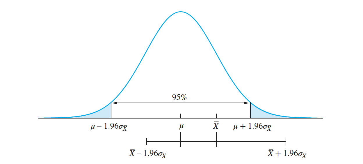
    • The middle $95\%$ of the curve, extending a distance $1.96 \sigma_{\overline X}$ on either side of population mean $\mu$, is indicated.

    • The interval $ \overline X \pm 1.96𝜎_{\overline X}$ is a $95\%$ confidence interval for the population mean $\mu$. It is clear that this interval covers the population mean $\mu$.

    • in this example, since the sample size is large, we may approximate $\sigma$ with the sample standard deviation $s = 0.1$

    • Therefore compute a $95\%$ confidence interval for the population mean fill weight $\mu$ to be $12.05 \pm (1.96)(0.01)$, or $(12.0304, 12.0696)$

    • Therefore a $68\%$ confidence interval for the mean fill weight of the boxes is $12.05 \pm (1.0)(0.01), or (12.04, 12.06)$.

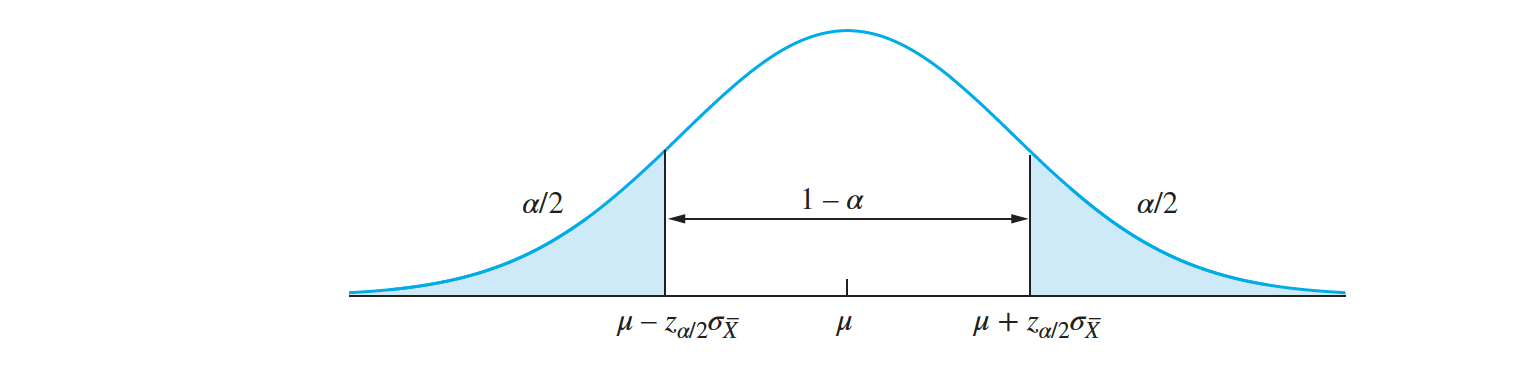
    • Let $X_1,\ldots, X_n$ be a large $(n > 30)$ random sample from a population with mean $\mu$ and standard deviation $\sigma$, so that $ \overline X$ s approximately normal. Then a level $100(1 − \alpha )\%$ confidence interval for 𝜇 is $ \overline X \pm z_\frac{\alpha}{2} \frac{\sigma}{\sqrt{n}}$ where $\sigma_{\overline X} = \frac {\sigma}{\sqrt n}$. When the value of $\sigma$ is unknown, it can be replaced with the sample standard deviation $s$.

    • In particular,

      • $\overline X \pm \frac {s}{\sqrt n}$ is a $68\%$ confidence interval for $\mu$.
      • $\overline X \pm 1.654 \frac {s}{\sqrt n}$ is a $90\%$ confidence interval for $\mu$.
      • $\overline X \pm 1.96 \frac {s}{\sqrt n}$ is a $95\%$ confidence interval for$\mu$.
      • $\overline X \pm 2.58 \frac {s}{\sqrt n}$ is a $99\%$ confidence interval for $\mu$.
      • $\overline X \pm 3 \frac {s}{\sqrt n}$ is a $99.7\%$ confidence interval for $\mu$.

  • For a given sample of size $N=70$, sample mean $ \overline{X } $= 408.2, the assumed standard standard deviation of the sample mean $\sigma_\overline{X} = $ 8.713217. Find an $80\%$ confidence interval.

• A team of geologists plans to measure the weights of $250$ rocks. After weighing each rock a large number of times, they will compute a $95\%$ confidence interval for its weight. Assume there is no bias in the weighing procedure. What is the probability that more than $240$ of the confidence intervals will cover the true weights of the rocks?

  

We have a simple random sample $X_{1}, …, X_{70}$ of strengths. The sample mean and standard deviation are $X = 408.20$ and $s = 72.9$. An engineer reported a confidence interval of $(393.86, 422.54)$ but neglected to specify the level.What is the level of this confidence interval. The population mean is unknown, and denoted by 𝜇.

• Determining the Sample Size Needed for a Confidence Interval of Specified Width

• It follows that the width of a confidence interval for a population mean based on a sample of size $n$ drawn from a population with standard deviation $\sigma$ is $ \mu \pm z_\frac{\alpha}{2} \frac{\sigma}{\sqrt{n}}$.
• If the confidence level $100(1−𝛼)\%$ is specified, we can look up the value $z_{\alpha∕2}$. If the population standard deviation $\sigma$ is also specified, we can then compute the value of $n$ needed to produce a specified width.

• The sample standard deviation of weights from $100$ boxes was $s = 0.1 oz$. How many boxes must be sampled to obtain a $99\%$ confidence interval of width $\pm 0.012 $?

• In the fill weight example discussed earlier in this section, the sample standard deviation of weights from $100$ boxes was $s = 0.1 ~ oz$. How many boxes must be sampled to obtain a $99\%$ confidence interval of width $\pm.012 ~oz$ ?

• One-Sided Confidence Intervals
  • Assume that a large sample has sample mean $\overline X$ and standard deviation $\sigma_{\overline X}$ . Figure shows how the idea behind the two-sided confidence interval can be adapted to produce a one-sided confidence interval for the population mean $\mu$. The normal curve represents the distribution of $\overline X$ . For $95\%$ of all the samples that could be drawn, $\overline X < 𝜇 + 1.645𝜎_{\overline X}$, and therefore the interval $(\overline X − 1.645𝜎_{\overline X} ,\infty)$ covers $\mu$.
  • This interval will fail to cover $\mu$ only if the sample mean is in the upper $5\%$ of its distribution. The interval $(\overline X −1.645𝜎_{\overline X},\infty)$ is a $95\%$ one-sided confidence interval for $\mu$, and the quantity $(\overline X + 1.645𝜎_{\overline X} ,\infty)$ is a $95\%$ lower confidence bound for $\mu$.

• Let $X_1,\ldots , X_n$ be a large $(n > 30)$ random sample from a population with mean $\mu$ and standard deviation $\sigma$, so that $X$ is approximately normal. Then a level $100(1 − \alpha)\%$ lower confidence bound for 𝜇 is $\overline{X} - z_{\alpha} { \sigma_{X}}$ and a level $100(1 − \alpha)\%$ upper confidence bound for $\mu$ is $\overline{X} + z_{\alpha} { \sigma_{X}}$ where $𝜎_X = \frac{𝜎}{\sqrt{ n}}$. When the value of $𝜎$ is unknown, it can be replaced with the sample standard deviation $s$.
• In particular,
  • $\overline X + 1.28 \frac {s}{\sqrt n}$ is a $90\%$ confidence interval for $\mu$.
  • $\overline X + 1.654 \frac {s}{\sqrt n}$ is a $95\%$ confidence interval for $\mu$.
  • $\overline X + 2.33 \frac {s}{\sqrt n}$ is a $99\%$ confidence interval for$\mu$.
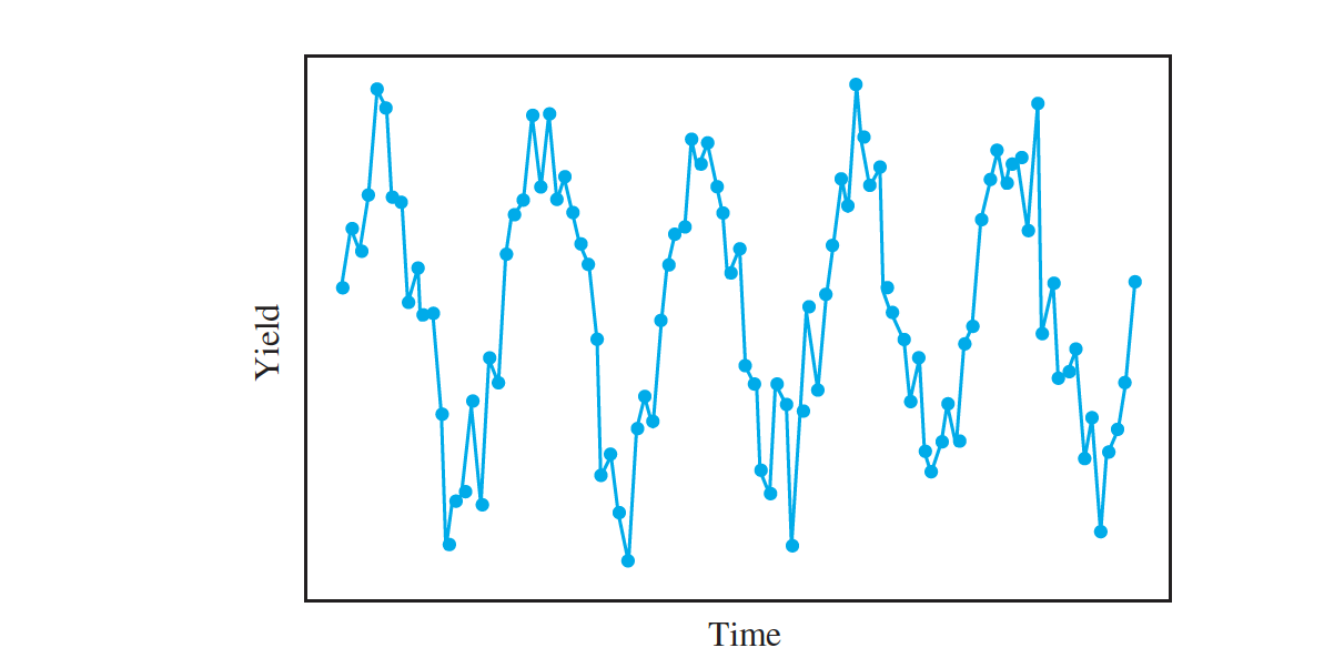
• Confidence Intervals Must Be Based on Random Samples
  • The methods described in this section require that the data be a random sample from a population. When used for other samples, the results may not be meaningful. Following are two examples in which the assumption of random sampling is violated.
  • We note that even for large samples, the distribution of $X$ is only approximately normal, rather than exactly normal. Therefore the levels stated for confidence intervals are approximate.
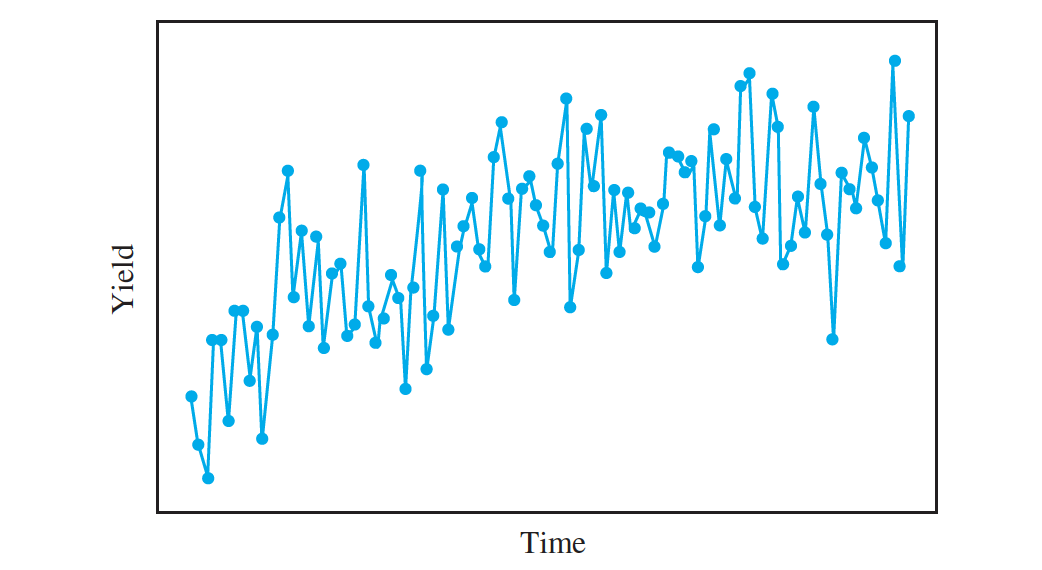
  • The engineer is studying the yield of another process. Below two figures presents yields from $100$ runs of this process, plotted against time. Should expression be used to compute a confidence interval for the mean yield of this process?