This post covers Introduction to probability from Statistics for Engineers and Scientists by William Navidi.

Basic Ideas

• Hypothesis Tests

  • A confidence interval is not quite what we need

  • The confidence interval does not directly tell us how confident we can be for hypothesis say that 𝜇 (population mean) > 11.

  • The statement “𝜇 > 11” is a hypothesis about the population mean 𝜇. To determine just how certain we can be that a hypothesis such as this is true, we must perform a

    hypothesis test.

  • A hypothesis test produces a number between $0$ and $1$ that measures the degree of certainty we may have in the truth of a hypothesis about a quantity such as a population mean or proportion. It turns out that hypothesis tests are closely related to confidence intervals. In general, whenever a confidence interval can be computed, a hypothesis test can also be performed, and vice versa

    • The population mean is actually greater than or equal to $100$, and the sample mean is lower than this only because of random variation from the population mean. Thus emissions will not go down if the new design is put into production, and the sample is misleading.
    • This is called the null hypothesis. In most situations, the null hypothesis says that the effect indicated by the sample is due only to random variation between the sample and the population.
    • The population mean is actually less than $100$, and the sample mean reflects this fact. Thus the sample represents a real difference that can be expected if the new design is put into production.
    • This explanation is called the alternate hypothesis. The alternate hypothesis says that the effect indicated by the sample is real, in that it accurately represents the whole population.

• Large-Sample Tests for a Population Mean (Null Hypothesis)

  • Let $X_{1},…, X_{n}$ be a large $(e.g., n > 30)$ sample from a population with mean $\mu$ and standard deviation $\sigma$. To test a null hypothesis of the form $H_0 : \mu ≤ \mu_{0}, H_0: \mu ≥ \mu_{0}$, or $ H_0: \mu = \mu_{0}$:

    • Compute the z-score: $z = \overline X − \mu_{0} \pm \sigma∕√n$. If $\sigma$ is unknown it may be approximated with $s$.

  • Compute the $P$-value. The $P$-value is an area under the normal curve, which depends on the alternate hypothesis as follows:

    Alternate Hypothesis $~~~~~~~~~~~~~~~~~~$ $P$-value

    $H_1 : \mu > \mu_{0}$ $~~~~~~~~~~~~~~~~~~$Area to the right of $z$

    $H_1: \mu < \mu_{0}$ $~~~~~~~~~~~~~~~~~~$Area to the left of $z$

    $H_1 : \mu ≠ \mu_{0}$ $~~~~~~~~~~~~~~~~~~$Sum of the areas in the tails cut off by $z$ and $−z$

  • A certain type of automobile engine emits a mean of $100$ mg of oxides of nitrogen $(NO_x)$ per second at $100$ horsepower. A modification to the engine design has been proposed that may reduce $NO_x$ emissions. The new design will be put into production if it can be demonstrated that its mean emission rate is less than $100$ mg/s. A sample of $50$ modified engines are built and tested. The sample mean $NO_x$ emission is $92$ mg/s, and the sample standard deviation is $21$ mg/s.

  • The null hypothesis is denoted $H_0$. The alternate hypothesis is denoted $H_1$. As usual, the population mean is denoted 𝜇. We have, therefore,

    $ H_0 : \mu ≥ 100 ~ versus ~ H_1 : \mu < 100$

  • The hypothesis test involves measuring the strength of the disagreement between the sample and $H_0$ to produce a number between $0$ and $1$, called a P-value.

  • If the P-value is sufficiently small, we may be willing to abandon our assumption that $H_0$ is true. This is referred to as rejecting the null hypothesis.

  • Thus we assume $ \mu = 100$. We do not know the population standard deviation $\sigma$. However, since the sample is large, we may approximate $\sigma$ with the sample standard deviation $s = 21$. Thus we have determined that under $H_0$, $\overline X$ has a normal distribution with mean $100$ and standard deviation $21∕ \sqrt 50 = 2.97$. The null distribution is $ \overline X ∼ N(100, 2.97^2)$.

  • The P-value is the probability that a number drawn from the null distribution would disagree with $H_0$ at least as strongly as the observed value of ,$\overline X$ which is $92$.

  • The P-value, therefore, is the probability that a number drawn from an $N(100, 2.97^2) $distribution is less than or equal to $92$.

    

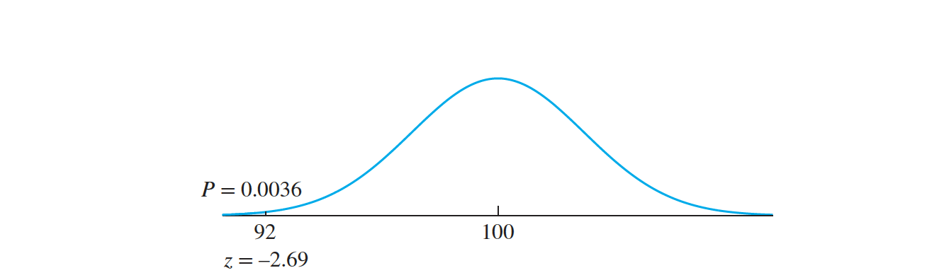
  • This probability is determined by computing the z-score:

    ​ $z = \frac{ 92 − 100}{2.97}$

    ​ $= −2.69$

  • In practice, events in the most extreme $0.36\% $ of their distributions very seldom occur. Therefore we reject $H_0$ and conclude that the new engines will lower emissions.

  • reject $H_0$ if $P ≤ 0.05$
  • Finally, note that the calculation of the P-value was done by computing a z-score. For this reason, the z-score is called a test statistic
  • We have mentioned that when assuming $H_0$ to be true, we use the value closest to $H_1$.
  • For example, in the emissions example just discussed, we are not specifically concerned with the possibility $\mu = 100$, but with the possibility $ \mu≥ 100$.
  • In one experiment, $45$ steel balls lubricated with purified paraffin were subjected to a $40$ kg load at $600$ rpm for $60$ minutes. The average wear, measured by the reduction in diameter, was $673.2$ 𝜇m, and the standard deviation was $14.9$ 𝜇m. Assume that the specification for a lubricant is that the mean wear be less than $675$ 𝜇m. Find the P-value for testing $H_0 : 𝜇 ≥ 675$ versus $H_1 :𝜇 < 675$.

• Drawing Conclusions from the Results of Hypothesis Tests

  • The smaller the P-value, the more certain we can be that $H_0$ is false.

  • The larger the P-value, the more plausible H0 becomes, but we can never

    be certain that $H_0$ is true.

  • A rule of thumb suggests to reject $H_0$ whenever $P ≤ 0.05$. While this rule is convenient, it has no scientific basis.

  • We rejected $H_0$; in other words, we concluded that $H_0$ was false. We did not reject $H_0$. However, we did not conclude that $H_0$ was true. We could only conclude that $H_0$ was plausible.

• Statistical Significance

  • Whenever the P-value is less than a particular threshold, the result is said to be “statistically significant” at that level. So, for example, if $P ≤ 0.05$, the result is statistically significant at the $5\%$ level;
  • If $P ≤ 0.01$, the result is statistically significant at the $1\%$ level, and so on. If a result is statistically significant at the $100𝛼\%$ level, we can also say that the null hypothesis is “rejected at level $100𝛼\%$.”
  • The $P$-value Is Not the Probability That $H_0$ Is True

• Tests for a Population Proportion

  • Let $X$ be the number of successes in n independent Bernoulli trials, each with success probability $p$; in other words, let $X ∼ Bin(n, p)$.

    To test a null hypothesis of the form $H_0 : p ≤ p_0, H_0 : p ≥ p_0, or H _0 : p = p_0$, assuming that both $np_0$ and $n(1 − p_0)$ are greater than $10$:

    Compute the z-score: $z =\hat p − p_0 \sqrt{\frac{ p_0(1 − p_0)}{n}}$

    .Compute the P-value. The P-value is an area under the normal curve,

    which depends on the alternate hypothesis as follows:

    Alternate Hypothesis $~~~~~~~~~~~~~~~~$P-value

    $H_1 : p > p_0$ $~~~~~~~~~~~~~~~~$Area to the right of z

    $H_1 : p < p_0$ $~~~~~~~~~~~~~~~~$Area to the left of z

    $H_1 : p ≠ p_0$ $~~~~~~~~~~~~~~~~$Sum of the areas in the tails cut off by z and −z

  • In courses on surveying, field work is an important part of the curriculum. The article reports that in a sample of $67$ students studying surveying, $45$ said that field work improved their ability to handle unforeseen problems. Can we conclude that more than $65\%$ of students find that field work improves their ability to handle unforeseen problems?

    Let $p$ denote the probability that a randomly chosen student believes that field work improves one’s ability to handle unforeseen problems. The null and alternate hypotheses are \(H_0 : p ≤ 0.65 ~vs. ~ H_1 : p > 0.65\)

    The sample proportion is \(\hat p = \frac{45}{67} = 0.6716\) Under the null hypothesis, $ \hat p$ is normally distributed with mean $0.65$ and standard deviation \(\sqrt{ \frac{ (0.65)(1 − 0.65)}{67}} =0.0583.\)

    The z-score is \(z = \frac{0.6716 − 0.6500}{0.0583} = 0.37\)

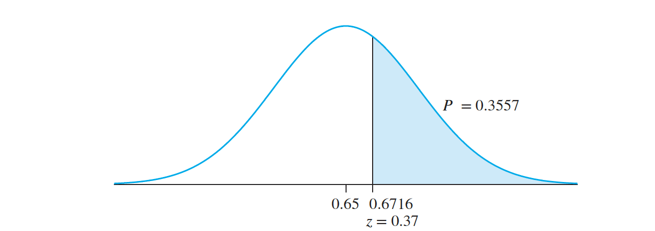
    The P-value is $0.3557$. We cannot conclude that more than $65\%$ of students find that field work improves their ability to handle unforeseen problems.

• Small-Sample Tests for a Population Mean

  • We described a method for testing a hypothesis about a population mean, based on a large sample.

  • A key step in the method is to approximate the population standard deviation $\sigma$ with the sample standard deviation $s$.

  • The normal curve is then used to find the $P$-value. When the sample size is small, $s$ may not be close to $\sigma$, which invalidates this large-sample method. However, when the population is approximately normal, the Student’s t distribution can be used.

  • Let $X_1,\ldots , X_n$ be a sample from a normal population with mean $\mu$ and standard

    deviation $\sigma$, where $\sigma$ is unknown.

    To test a null hypothesis of the form $H_0 : \mu ≤ \mu_0, H_0 : \mu ≥ \mu_0, or ~ H_0 : \mu = \mu_0$:

    Compute the test statistic $t = \frac { \overline X − \mu_0} {s∕ \sqrt n}$.

    Compute the $P$-value. The $P$-value is an area under the Student’s t curve with $n − 1$ degrees of freedom, which depends on the alternate hypothesis as follows:

    Alternate Hypothesis $~~~~~~~~~$P-value

    $H_1 : \mu > \mu_0$ $~~~~~~~~~$Area to the right of t

    $H_1 : \mu < \mu_0$ $~~~~~~~~~$Area to the left of t

    $H_1 : \mu \neq \mu_0$ $~~~~~~~~~$Sum of the areas in the tails cut off by t and −t

    If $\sigma$ is known, the test statistic is $z = \frac { \overline X − \mu_0}{\sigma∕ \sqrt n}$, and a $z$ test should be performed.

  • Spacer collars for a transmission counter shaft have a thickness specification of $38.98–39.02 ~ mm$. The process that manufactures the collars is supposed to be calibrated so that the mean thickness is $39.00$ mm, which is in the center of the specification window. A sample of six collars is drawn and measured for thickness. The six thicknesses are $39.030, 38.997, 39.012, 39.008, 39.019, ~ and ~39 .002$. Assume that the population of thicknesses of the collars is approximately normal. Can we conclude that the process needs recalibration?

    Denoting the population mean by 𝜇, the null and alternate hypotheses are \(H_0 : \mu = 39.00 ~ versus ~ H_1 : \mu ≠ 39.00\)

    In this example the observed values of the sample mean and standard deviation are $ \overline X = 39.01133$ and $s = 0.011928$. The sample size is $n = 6$. The null hypothesis specifies that $\mu = 39$. The value of the test statistic is therefore \(t = \frac {39.01133 − 39.000}{.011928∕ \sqrt 6}= 2.327\) The P-value is the probability of observing a value of the test statistic whose disagreement with $H_0$ is as great as or greater than that actually observed. Since $H_0$ specifies that $\mu = 39.00$, this is a two-tailed test, so values both above and below $39.00 $ disagree with $H_0$. Therefore the $P$-value is the sum of the areas under the curve corresponding to $t > 2.327$ and $t < −2.327$.

    

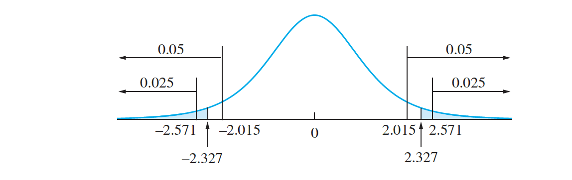
    Thus the P-value is between 0.05 and 0.10. It would be prudent to recalibrate.

• Large-Sample Tests for the Difference Between Two Means

  • Let $X_1,…, X_{n_X}$ and $Y_1,…, Y_{n_Y}$ be large (e.g., $n_X > 30$ and $n_Y > 30$) samples from populations with means $\mu_X$ and $\mu_Y$ and standard deviations $\sigma_X$ and $\sigma_Y$, respectively. Assume the samples are drawn independently of each other.

    To test a null hypothesis of the form

    \[H_0 : \mu_X −\mu_Y ≤ \Delta_0, H_0 : \mu_X −\mu_Y ≥ \Delta_0, or ~ H_0: \mu_X − \mu_Y = \Delta_0\]

    Compute the z-score: \(z = \frac {( \overline X − \overline Y)−\Delta_0 }{\sqrt{ (\sigma^2_X∕n_X + \sigma^2_Y∕n_Y)}}\) .If $\sigma_X$ and $\sigma_Y$ are unknown they may be approximated with $s_X$ and $s_Y$ , respectively. Compute the $P$-value. The $P$-value is an area under the normal curve, which depends on the alternate hypothesis as follows:

    Alternate Hypothesis $~~~~~~~~~~~~~~$$P$-value

    $H_1 : \mu_X − \mu_Y > \Delta_0$ $~~~~~~~~~~~~~~$Area to the right of z

    $H_1 : \mu_X − \mu_Y < \Delta_0$ $~~~~~~~~~~~~~~$Area to the left of z

    $H_1 : \mu_X − \mu_Y ≠ \Delta_0$ $~~~~~~~~~~~~~~$Sum of the areas in the tails cut off by z and −z

  • To investigate this concern, she samples $120$ ball bearings that were manufactured early in the morning, before the shop was fully heated, and finds their mean diameter to be $5.068$ mm and their standard deviation to be $0.011$ mm. She independently samples $65$ ball bearings manufactured during the afternoon and finds their mean diameter to be $5.072$ mm and their standard deviation to be $0.007$ mm. Can she conclude that ball bearings manufactured in the morning have smaller diameters, on average, than ball bearings manufactured in the afternoon?

    The sample sizes are $n_X = 120$ and $n_Y = 65$. We are interested in the difference $\mu_X − \mu_Y$.

    The observed values are $ \overline X = 5.068$ and $ \overline Y = 5.072$ for the sample means, and $s_X = 0.011$ and $s_Y = 0.007$ for the sample standard deviations. Under $H_0, \mu_X − \mu_Y = 0 $ (the value closest to $H_1$). We approximate the population variances $\sigma^2_X$ and $𝜎^2_Y$ with the sample variances $s^2_X = 0.0112$ and $s^2_Y = 0.0072$, respectively, and substitute $n_X = 120$ and $n_Y = 65$ to compute the standard deviation of the null distribution

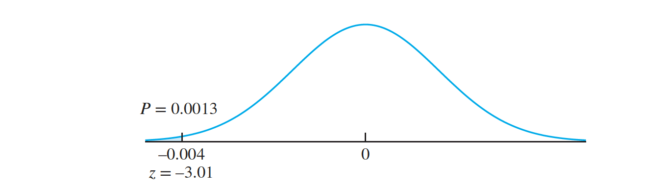    \(\sqrt {0.0112∕120 + 0.0072∕65} = 0.001327\) . The null distribution of $ \overline X − \overline Y$ is therefore \(\overline X − \overline Y ∼ N(0, 0.001327^2)\) The observed value of $ \overline X − \overline Y$ is $5.068 − 5.072 = −0.004$. The z-score is \(z = \frac {−0.004 − 0}{0.001327}= −3.01\)

    Figure shows the null distribution and the location of the test statistic. The $P$-value is 0.0013. The manager’s suspicion is correct.

    The bearings manufactured in the morning have a smaller mean diameter.

    Note that we used the assumption that the samples were independent when computing the variance of $ \overline X − \overline Y$.

    This is one condition that is usually easy to achieve in practice.

    Unless there is some fairly obvious connection between the items in the two samples, it is usually reasonable to assume they are independent.

  • The data will consist of two samples, one from each population. If the difference is far from $0$, we will conclude that the population means are different. If the difference is close to $0$, we will conclude that the population means might be the same.

• Tests for the Difference Between Two Proportions

  • Let $X ∼ Bin(n_X, p_X)$ and let $Y ∼ Bin(n_Y, p_Y )$. Assume that there are at least

    $10$ successes and $10$ failures in each sample, and that X and Y are independent.

    To test a null hypothesis of the form \(H_0 : p_X − p_Y ≤ 0, H_0 : p _X − p_Y ≥ 0, or ~ H_0 : p_X − p_Y = 0\)

    • Compute

      ​
      \(\hat p_X = \frac{X}{n_X}, \hat p_Y = \frac{Y}{n_Y}, and ~ \hat p = \frac{X + Y}{n_X + n_Y}\)

    • Compute the z-score: \(z = \frac{\hat p_X − \hat p_Y}{\hat p(1 − \hat p)(1∕n_X + 1∕n_Y )}\)

    • Compute the P-value. The P-value is an area under the normal curve,

      Which depends on the alternate hypothesis as follows:

    Alternate Hypothesis $~~~~~~~~~~~~~~~~~~~$ P-value

    $H_1 : p_X − p_Y > 0$ $~~~~~~~~~~~~~~~~~~~$Area to the right of z

    $H_1 : p_X − p_Y < 0$ $~~~~~~~~~~~~~~~~~~~$Area to the left of z

    $H_1 : p_X − p_Y ≠ 0$ $~~~~~~~~~~~~~~~~~~~$Sum of the areas in the tails cut off by $z$ and $−z$

  • A mobile computer network consists of computers that maintain wireless communication with one another as they move about a given area. A routing protocol is an algorithm that determines how messages will be relayed from machine to machine along the network, so as to have the greatest chance of reaching their destination. The article compares the effectiveness of two routing protocols over a variety of metrics, including the rate of successful deliveries. Assume that using protocol A, 200. messages were sent, and 170 of them, or 85%, were successfully received. Using protocol B, 150 messages were sent, and 123 of them, or 82%, were successfully received. Can we conclude that protocol A has the higher success rate?

  • The random variables $X$ and $Y$ have binomial distributions, with $n_X = 200$ and $n_Y = 150$ trials, respectively. The success probabilities are $p_X$ and $p_Y$. The observed values of the sample proportions are $ \hat p_X = 170∕200 = 0.85$ and $ \hat p_Y = 123∕150 = 0.82$.

    The null and alternate hypotheses are \(H_0 : p_X − p_Y ≤ 0 ~ versus ~ H_1 : p_X − p_Y > 0\) Therefore we must estimate them both population proportions with a common value. The appropriate value is the pooled proportion, obtained by dividing the total number of successes in both samples by the total sample size. \(\hat p = \frac {X + Y} {n_X + n_Y}\) The null distribution of $ \hat p_X- \hat p_Y$ is therefore estimated by substituting the pooled proportion $\hat p$ for both $p_X$ and $p_Y$ into expression. This yields \(\hat p_X − \hat p_Y ∼ N(0,\hat p(1 − \hat p)(\frac {1}{n_X}+ \frac {1}{n_Y}))\)

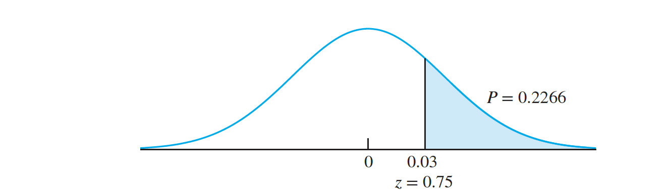
    In this example, $ \hat p = \frac {(170 + 123)}{(200 + 150)} = 0.837$. Under $H_0$, we take $p_X − p_Y = 0$. The null distribution of $ \hat p_X −\hat p_Y$ is therefore normal with mean $0$ and standard deviation

    $ \sqrt {0.837(1 − 0.837)(1∕200 + 1∕150)} = 0.0399$. The observed value of $ \hat p_X- \hat p_Y$

    is $0.85 − 0.82 = 0.03$. The z-score is therefore \(z = \frac {0.03 − 0}{0.0399} = 0.75\) On the basis of this P-value, we cannot conclude that protocol B has the greater success rate.

• Small-Sample Tests for the Difference Between Two Means

  • Let $X_1,…, X_{n_X}$ and $Y_1,…, Y_{n_Y}$ be samples from normal populations with means $\mu_X$ and $\mu_Y$ and standard deviations $ \sigma_X$ and $ \sigma_Y$ , respectively. Assume the samples are drawn independently of each other. If $𝜎_X$ and $𝜎_Y$ are not known to be equal, then, to test a null hypothesis of the form \(H_0 : \mu_X − \mu_Y ≤ \Delta_0, H_0 : \mu_X − \mu_Y ≥ \Delta_0, ~ or ~H_0 : \mu_X − \mu_Y = \Delta_0\)

  • Compute \(𝜈 = \frac{[(s^2_X∕n_X) + (s^2_Y∕n_Y )]^2}{[(s^2_X∕n_X)^2∕(n_X − 1)] + [(s^2_Y∕n_Y )^2∕(n_Y − 1)]}\) ,rounded downto the nearest integer.

  • Compute the test statistic

    \[t = \frac{(\overline X − \overline Y)−\Delta_0}{ \sqrt {s^2_X∕n_X + s^2_Y∕n_Y}}\]

  • Compute the P-value. The P-value is an area under the Student’s t curve with $𝜈$ degrees of freedom, which depends on the alternate hypothesis as follows:

    Alternate Hypothesis $~~~~~~~~~~~~~~~~~~~~~~~$P-value

    $H_1 : 𝜇_X − 𝜇_Y > \Delta_0$ $~~~~~~~~~~~~~~~~~~~~~~~$Area to the right of $t$

    $H_1 : \mu_X − \mu_Y < \Delta_0$ $~~~~~~~~~~~~~~~~~~~~~~~$Area to the left of $t$

    $H_1 : \mu_X − \mu_Y \neq \Delta_0$ $~~~~~~~~~~~~~~~~~~~~~~~$Sum of the areas in the tails cut off by $t$ and $−t$

  • The t test can be used in some cases where samples are small, and thus where the Central Limit Theorem does not apply. We present an example.

  • Assume that in six identically prepared specimens without the enzyme present, the numbers of molecules counted are $33, 30, 26, 22, 37, ~ and ~ 34$. Assume that in four identically prepared specimens with the enzyme present, the counts were $22, 29, 25, ~ and ~ 23$. Can we conclude that the counts are lower when the enzyme is present?

    The null and alternate hypotheses are \(H_0 : \mu_X − \mu_Y ≤ 0 ~ versus ~ H_1 : \mu_X − \mu_Y > 0\) The observed values for the sample means and standard deviations are $ \overline X = 30.333, \overline Y = 24.750, s_X = 5.538, and ~ s_Y = 3.096$. The sample sizes are $n_X = 6 $and $n_Y = 4$. Substituting the values for the sample standard deviations and sample sizes, we compute $\nu = 7.89$, which we round down to $7$. Under $H_0, \mu_X − \mu_Y = 0$.

    The test statistic is therefore \(t = \frac{(\overline X − \overline Y) − 0}{\sqrt{s^2_X∕n_X + s^2_Y∕n_Y}}\) Under $H_0$, the test statistic has a Student’s t distribution with seven degrees of freedom. Substituting values for $\overline X, \overline Y, s_X, s_Y , n_X, ~ and ~n_Y,$ we compute the value of the test statistic to be \(t = \frac {5.583 − 0}{2.740} = 2.038\)

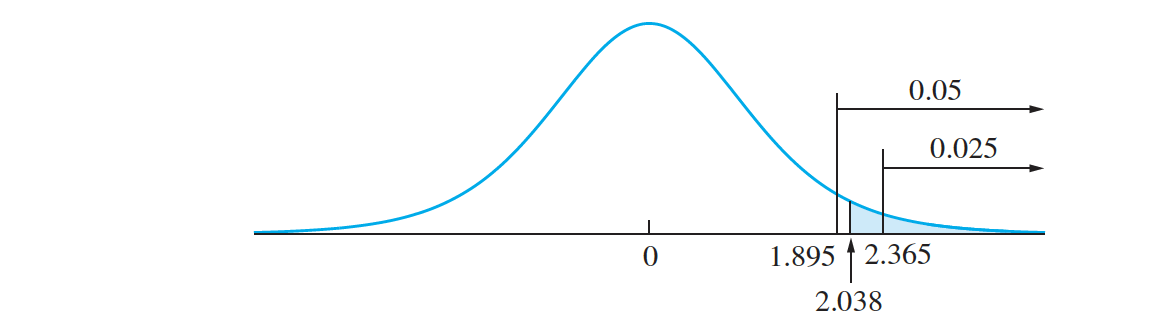
    Consulting the t table with seven degrees of freedom, we find that the value cutting off $5\%$ in the right-hand tail is $1.895$, and the value cutting off $2.5\%$ is $2.365$. The P-value is therefore between 0.025 and 0.05.We conclude that the mean count is lower when the enzyme is present.

• Tests with Paired Data

  • We treat the collection of differences as a single random sample from a population of differences. Denote the population mean of the differences by $\mu_D$ and the standard deviation by $\sigma_D$. There are only eight differences, which is a small sample. If we assume that the population of differences is approximately normal,

  • Let $(X_1, Y_1),…, (X_n, Y_n)$ be a sample of ordered pairs whose differences $D_1,\ldots, D_n$ are a sample from a normal population with mean $\mu_D$. Let $s_D$ be the sample standard deviation of $D_1,\ldots, D_n$.

    To test a null hypothesis of the form \(H_0 : \mu_D ≤ \mu_0, H_0 : \mu_D ≥ \mu_0, or, H_0 : \mu_D = \mu_0\) Compute the test statistic \(t = \frac { \overline D − \mu_0} {s_D∕√ n}\)

  • Compute the P-value. The P-value is an area under the Student’s t curve with $n − 1$ degrees of freedom, which depends on the alternate hypothesis as follows:

    Alternate Hypothesis $~~~~~~~~~~~~~~~~~~~~~~~~~$P-value

    $H_1 : \mu_D > \mu_0$ $~~~~~~~~~~~~~~~~~~~~~~~~~$Area to the right of t

    $H_1 : \mu_D < \mu_0$ $~~~~~~~~~~~~~~~~~~~~~~~~~$Area to the left of t

    $H_1 : \mu_D ≠ \mu_0$ $~~~~~~~~~~~~~~~~~~~~~~~~~$Sum of the areas in the tails cut off by $t$ and $−t$

    If the sample is large, the $D_i$ need not be normally distributed, the test statistic is \(z = \frac{ \overline D − \mu_0}{s_D∕\sqrt n}\) , and a $z$ test should be performed.

  • Particulate matter (PM) emissions from automobiles are a serious environmental concern. Eight vehicles were chosen at random from a fleet, and their emissions were measured under both highway driving and stop-and-go driving conditions. The differences (stop-and-go emission − highway emission) were computed as well. The results, in milligrams of particulates per gallon of fuel, were as follows:

    

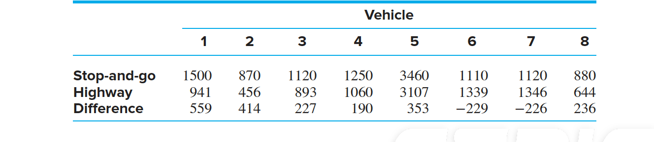
    we can use, The observed value of the sample mean of the differences is $D = 190.5$. The sample standard deviation is $s_D = 284.1$. The null and alternate hypotheses are \(H_0 : \mu_D ≤ 0 ~ versus ~ H_1 : \mu_D > 0\)

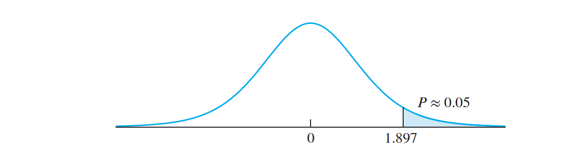
    The test statistic is \(\begin{align*} t &= \frac {D − 0}{s_D∕\sqrt n} \\ &= \frac{190.5 − 0}{ {284.1} / {\sqrt 8}} \\ &= 1.897 \\ \end{align*}\)

  • The null distribution of the test statistic is Student’s t with seven degrees of freedom. Figure presents the null distribution and indicates the location of the test statistic. This is a one-tailed test. The t table indicates that $5\%$ of the area in the tail is cut off by a t value of $1.895$, very close to the observed value of $1.897$.

  • The $P$-value is approximately $0.05$.

  • Note that the $95\%$ lower bound is just barely consistent with the alternate hypothesis. This indicates that the P-value is just barely less than $0.05$