Correlation and regression

6 minute read

Published: November 05, 2021

This post covers Introduction to probability from Statistics for Engineers and Scientists by William Navidi.

Basic Ideas

Correlation and linear regression
- The methods of correlation and simple linear regression are used to analyze bivariate data in order to determine whether a straight line fit is appropriate,
- to compute the equation of the line if appropriate, and to use that equation to draw inferences about the relationship between the two quantities.
- The correlation coefficient as a way of describing how closely related two physical
  characteristics are.
- We define the correlation coefficient, which is a numerical measure of the strength of the linear relationship between two variables. The correlation coefficient is usually denoted by the letter r.
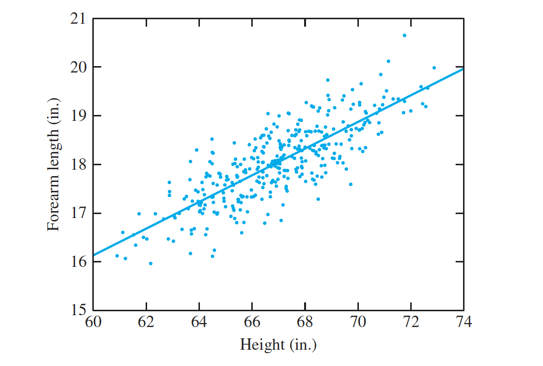
- We say that there is a positive association between height and forearm length. The slope is approximately constant throughout the plot, indicating that the points are clustered around a straight line.
- The line superimposed on the plot is a special line known as the least-squares line.
- The degree to which the points in a scatterplot tend to cluster around a line reflects the
  strength of the linear relationship between x and y.
- Changing the scale of the axes can make the clustering appear tighter or looser. For this reason, we define the correlation coefficient, which is a numerical measure of the strength of the linear relationship between two variables.
- Let $(x_1, y_1),…, (x_n, y_n)$ represent $n$ points on a scatterplot. To compute the correlation, first compute the means and standard deviations of the $x_s$ and $y_s$, that is, $ \overline x, \overline y, s_x, and s_y$.
- Then convert each $x$ and $y$ to standard units, or, in other words, compute the z-scores: $(x_i − \overline x)∕s_x, (y_i − \overline y)∕s_y$. The correlation coefficient is the average of the products of the $z-scores$, except that we divide by $n − 1$ instead of $n$:
  \[r = \frac{1}{n − 1} \Sigma_{i=1}^{n}( \frac{x_i − \overline x} {s_x})( \frac {y_i − \overline y} {s_y})\\\]
  We can rewrite Equation (1) in a way that is sometimes useful. By substituting $ \sqrt {\Sigma_{i=1}^n (x_i − \overline x)^2∕(n − 1)}$ for $s_x$ and $ \sqrt{ \Sigma_{i=1}^n(y_i − \overline y)^2∕(n − 1)}$ for $s_y$, we obtain
  \[r = \frac{ \Sigma^n_{i=1}(x_i − \overline x)(y_i − \overline y)}{\sqrt{ \Sigma_{i=1}^n(x_i − \overline x)^2}{\sqrt{ \Sigma_{i =1}^n(y_i − \overline y)^2}}}\\\]
  By performing some algebra on the numerator and denominator, we arrive at yet another equivalent formula for r:
  \[r = \frac {\Sigma_{i =1}^n x_iy_i − n \overline x \overline y}{\sqrt {\Sigma_{i=1}^n x^2_i − n \overline x^2} \sqrt {\Sigma_{i=1}^n y^2_i− n \overline y^2}}\\\]
- In principle, the correlation coefficient can be calculated for any set of points. In many cases, the points constitute a random sample from a population of points.
- In these cases the correlation coefficient is often called the sample correlation, and it is an estimate of the population correlation.
- In Population correlation, you may imagine the population to consist of a large finite collection of points, and the population correlation to be the quantity computed using on the whole population, with sample means replaced by population means.
- The sample correlation can be used to construct confidence intervals and perform hypothesis tests on the population correlation; these will be discussed later in this section.
- Finally, a bit of terminology: Whenever $r ≠ 0$, $x$ and $y$ are said to be correlated. If $r = 0, x$ and $y$ are said to be uncorrelated.
How the Correlation Coefficient Works
- In the first quadrant, the z-scores $(x_i− \overline x)∕s_x$ and $(y_i− \overline y)∕s_y$ are both positive, so their product is positive as well.
- If the plot had a negative slope, there would be more points in the second and fourth quadrants, and the correlation coefficient would be negative.
- But since the correlation coefficients have no units, they are directly comparable, and therefore, we can conclude that the relationship between heights of men and their forearm lengths is more strongly linear than the relationship between temperature and humidity.
The Correlation Coefficient Measures Only Linear Association
- The value of y is determined by $x$ through the function $y = 64x − 16x^2$. Yet the correlation between $x$ and $y$ is equal to $0$
- The value of $0$ for the correlation indicates that there is no linear relationship between x and y, which is true
- The lesson of this example is that the correlation coefficient should only be used when the relationship between the x and y is linear. Otherwise the results can be misleading.
The Correlation Coefficient can be Misleading when Outliers are Present
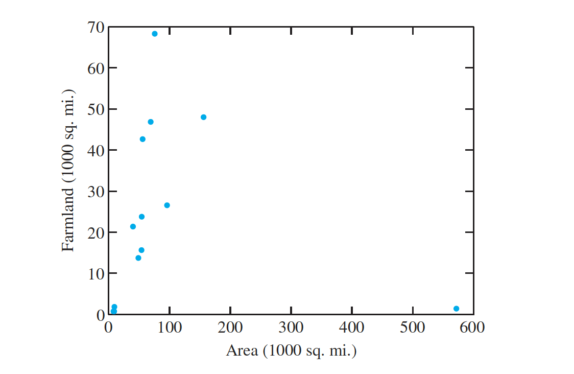
- In general, states with larger land areas have more farmland.
- The major exception is Alaska, which has a huge area but very little farmland.
Controlled Experiments Reduce the Risk of Confounding
- In controlled experiments, confounding can often be avoided by choosing values for factors in a way so that the factors are uncorrelated.
- Observational studies are studies in which the values of factors cannot be chosen
  by the experimenter
- Because confounding is difficult to avoid, observational studies must generally be repeated a number of times, under a variety of conditions, before reliable conclusions can be drawn.
Inference on the Population Correlation
- Let $X$ and $Y$ be random variables with the bivariate normal distribution.
  Let 𝜌 denote the population correlation between X and Y. Let $(x_1, y_1),…, (x_n, y_n)$ be a random sample from the joint distribution of $X$ and $Y$.
- Let r be the sample correlation of the n points.Then the quantity $W = \frac{1}{2} ln \frac {1 + r}{1 − r }\\$ is approximately normally distributed, with mean given by $\mu_W = \frac{1}{2}ln \frac{1 + 𝜌}{1 − 𝜌}\\$ and variance given by $𝜎^2_W= \frac{1}{n − 3}\\$ Note that $\mu_W$ is a function of the population correlation 𝜌. To construct confidence intervals, we will need to solve Equation for $\rho$. $\rho = \frac {e^2_{\mu_W} − 1}{ e^2_{\mu_W} + 1}$
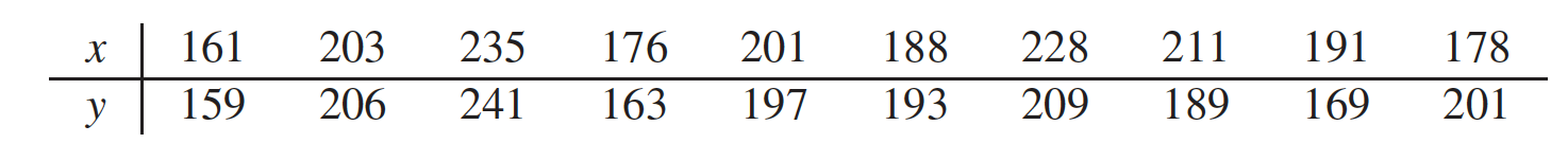
In a study of reaction times, the time to respond to a visual stimulus $(x)$ and the time to respond to an auditory stimulus $(y)$ were recorded for each of $10$ subjects. Times were measured in ms. The results are presented in the following table.